

Photochemistry_of_Organic
.pdfFlash Photolysis |
95 |
The duration of the pump pulse is the main factor that limits the time resolution of flash photolysis. The commonly used specification of full width at half-height (FWHH) is incomplete, since the shape of many pulses is far from Gaussian. Tailing and afterglow of, for example, conventional discharge flash lamps and excimer lasers can severely reduce the time resolution achievable. Only a few groups still use the so-called conventional apparatus, that is, flash photolysis systems pumped by a discharge flash lamp of microsecond duration. Yet these instruments still give the best performance on the millisecond time scale and the whole setup costs a fraction of that of a laser. Tremendous developments in the production of short laser pulses, in the time resolution and sensitivity of detectors, the speed and dynamic range of digitizers and the speed and memory capacities of computers (statistical averaging) have improved time resolution down to femtoseconds.
Most flash photolysis systems with excitation pulses of nanosecond and longer duration operate in the kinetic mode, that is, the transient absorption is monitored at a single wavelength as a function of time. Spectrographic detection can be done using gated microchannel plates as light shutters (and amplifiers) and diode-array detectors, which provide digitized transient absorption spectra at a given time delay with respect to the laser pulse. Basically, both techniques probe one-dimensional slices of the same physical information that consists of a two-dimensional array A of absorbances A(l,t) as a function of wavelength l and time t after excitation (Figure 2.18). Systems with shorter excitation pulses and subnanosecond time resolution usually operate in the spectrographic mode (pump–probe spectroscopy). The analysis of kinetic and spectrographic data is described in Sections 3.7.4 and 3.7.5.
Beware of artefacts! This cautionary remark should always be kept in mind when carrying out flash photolysis. Stray light and fluorescence, acoustic shock waves and inhomogeneous transient distributions produced in the sample by focused laser pulses, extraneous electronic pulses from flash lamps or Q-switches, signal echoes and the like often distort the transient waveforms or spectra.
3.7.1Kinetic Flash Photolysis
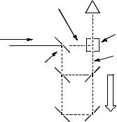
Flash photolysis setups (Figure 3.14) are single-beam instruments that measure absorbance changes in time.
short-lived pump pulse (laser)
continuous light source
photomultiplier
sample cell 
 mono- chromator
|
|
|
|
|
|
|
|
|
|
|
|
|
|
|
|
|
|
|
|
|
|
|
|
|
|
|
|
|
|
|
|
|
|
|
|
|
|
|
|
|
|
|
|
|
|
|
|
|
|
|
|
|
|
|
|
|
|
|
|
|
|
|
|
|
|
|
|
|
|
|
|
|
|
|
|
|
|
|
|
|
|
|
|
|
|
|
|
|
|
|
|
|
digital transient recorder |
||
|
data analysis |
|
|
|
|
|
|||||
Figure 3.14 Kinetic setup for flash photolysis
96 |
Techniques and Methods |
Depending on the pulsed excitation source, but also on the optical arrangement (excitation parallel or vertical to the monitoring light) and focusing optics, the concentrations of generated transients may differ widely. Strictly parallel orientation of the pump and probe beams is avoided to inhibit the strong pump pulse from hitting the detector of the probe beam. Both orientations have some advantages and it is useful to devise the detection system such that it can be switched from one geometry to the other. An advantage of right-angle excitation with diffuse pump beams is the relatively low concentration of transient intermediates produced in the sample. This reduces the half-life of bimolecular reactions between transient intermediates such as triplet–triplet annihilation or radical recombination. Sensitivity can be maintained by collecting transient absorbance over an extended optical pathlength; pathlengths of 4 cm are conveniently used with excimer lasers and 10–20 cm with conventional discharge flashlamps. An advantage of parallel pump and probe beams is that the sample absorbance can be raised to a point where essentially all of the exciting light is absorbed.
With nonexponential decay traces, it may be difficult to distinguish between secondorder reactions and two overlapping first-order decays with similar rate constants. In such cases, it is helpful to change the initial concentration of the transient intermediates either by reducing the concentration of the reactant or the intensity of the excitation pulse or by switching from parallel to right-angle excitation. Second-order decays will then exhibit longer half-lives, while the sum of first-order decays remains the same.
Flash photolysis commonly produces transient concentrations that are unevenly distributed. Inhomogeneity arises from hot spots in the laser beam profile, focusing optics, internal filter effects in the sample solutions and imperfect overlap between the volume excited by the pump beam and that analysed by the probe beam. Inhomogeneous sample distributions distort kinetic traces196 and should be minimized, even at the expense of some loss in the signal intensity. A gradient in the concentration at right-angles to the monitoring beam will distort even the traces of first-order reactions, since the average absorbance of such a solution will not be proportional to the average transient concentration. The absorbance at the excitation wavelength should be kept below about 0.5 at the excitation wavelength with vertical excitation. The effect of inhomogeneous sample distributions for a given setup can be determined by observing a strongly absorbing transient intermediate such as the triplet of 9,10-dibromoanthracene in aerated solution that is known to give a clean first-order decay. Inhomogeneous transient distributions are manifested by a sigmoid distortion of the decay traces. When the transient absorption is monitored parallel to the excitation beam, inhomogeneous transient distributions are less distorting, so that much higher sample concentrations can be used.
A common procedure in mechanistic studies is to follow the growth or decay rate of a transient intermediate as a function of the concentration of some other species such as a sensitizer, quencher, trapping agent, acid or buffer. Bimolecular rate constants are then obtained from the concentration dependence of the observed first-order rate constants, kobs (see Section 3.9.7).
Good kinetic data are usually reproducible within a few percent. Standard errors determined from fitting of a single trace are commonly even smaller, but reproducibility should be judged from the analysis of several decay traces, because systematic errors, such as instability of the monitoring light source over the period of observation or variations of temperature, do not show in a single trace. The temperature dependence of the logarithm

Flash Photolysis |
97 |
of first-order rate constants obeying Arrhenius law is proportional to the activation energy Ea, dlog(k/s 1)/dT ¼ Ea/(2.3RT2). Hence fast reactions having low activation energies are generally not very sensitive to temperature changes. Nevertheless, assuming A ¼ 1013 s 1, one predicts a 5% increase for a rate constant of 106 s 1 when the temperature increases by 1 C around ambient temperature. Hence sample cells should be held in a thermostat if highly accurate kinetic data are required.
Digitizing oscilloscopes with sampling rates of 1 gigasample s 1 and high-bandwidth amplifiers ( 500 MHz) nicely match the time resolution required to see the fastest processes resolvable by excitation with Q-switched lasers, excimer lasers or dye lasers, which have pulse widths on the order of 2–20 ns. The high storage depth of modern digitizers provides access to long delay times even at high time resolution so that both fast and slow processes may be captured in a single trace. Furthermore, the pre-trigger capturing facility of these devices obviates the need for trigger cascades. Jitter is largely eliminated when the trigger is generated directly from the laser pulse with a photodiode.
3.7.2Spectrographic Detection Systems
The photographic plates or film used in the early days to record the absorption spectra of transient intermediates have been replaced by diode arrays. The time window during which the transient spectra are collected can be determined by employing a short probe pulse of light. Alternatively, microchannel plate image intensifiers placed in front of the diode arrays may be used in combination with continuous monitoring light sources to achieve nanosecond time windows; image intensifiers not only enhance the intensity of the monitoring light during the active time window, but also act as shutters with a (de-)activation rise time of about 1 ns and an on:off transmission ratio >106. Such an effective shutter is required if the monitoring light source is continuous during the long integration times of the detectors ( 30 ms). Cut-off filters that do not transmit below the cut-off wavelength should be used for protection of the detector from the excitation pulse and to eliminate second-order reflections from the grating. When excess monitoring light is available at some wavelengths, compensating filter solutions may be adjusted with appropriate dyes to equalize the spectral distribution of the source. A commercially available setup for nanosecond laser flash photolysis (LFP) is shown in Figure 3.15.
Fluorescence will interfere with kinetic absorbance measurements for the duration of the fluorescence or of the pump pulse, whichever is longer. Scattered light and
Figure 3.15 Spectrographic setup for nanosecond LFP. Reproduced by permission of Applied Photophysics Ltd
98 |
Techniques and Methods |
fluorescence can easily drown the monitoring light source because the intensity of the pump pulse is commonly orders of magnitude higher than that of the probe pulse or of the continuous monitoring light source. Stray light problems are reduced by using appropriate filters, by pulsing the monitoring lamp and by taking advantage of the different angular dispersion of scattered light and the monitoring beam.
When the observation wavelength lies within the absorbance of the reactant, negative absorption may be due to bleaching. Transient kinetics should always be determined at several wavelengths and transient spectra at various delay times, t.
Streak cameras allow one to probe the entire two-dimensional array A(l,t) following excitation with a single pulse. They are, however, rarely used for pump–probe flash photolysis because of their low precision and high price. Repeated excitation is necessary to probe different wavelengths on a kinetic apparatus and different time delays on spectrographic devices. Variations of the pump pulse intensity will affect the spectral information determined point-by-point in the kinetic mode and the kinetic information derived from sequential spectra. Systematic variations of the instrument performance or decomposition of the sample with time can easily produce artificial kinetics in the spectrographic mode and artificial spectral features in the kinetic mode, respectively. It is, of course, best to determine and eliminate the source of such problems. Notwithstanding, probing at different wavelengths or time delays should always be done at random rather than in an ordered sequence; if systematic variations occur during data collection (commonly 10 min to 1 h), they will produce an increase in random noise rather than artefacts such as distorted kinetics.
Fluctuations of the laser pulse can be eliminated by calibration, that is, by independent monitoring of the pulse intensity for each individual shot. Sample degradation can be avoided by using flow systems.
3.7.3Pump–Probe Spectroscopy
Lasers with ultrashort pulse lengths down to a few femtoseconds (1 fs ¼ 10 15 s) are now available commercially. However, photomultipliers and the associated electronic digitizers are not sufficiently fast to follow waveforms much below 1 ns. Therefore, devices with picoand femtosecond time resolution use optical delay lines to define the time delay between the excitation pulse and the probe pulse (Figure 3.16). By focusing part of the
pump pulse |
detector |
|
|
laser pulse |
probe cell |
|
|
|
delayed probe |
|
pulse |
semitransparent |
|
mirror |
|
|
movable delay line |
Figure 3.16 Conceptual design of a pump–probe apparatus

Flash Photolysis |
99 |
pump pulse into a solution or a CaF2 plate, a broad supercontinuum (300–700 nm) is generated, which can be used as the probe pulse in pump–probe spectroscopy.194 A pathlength difference of 0.3 mm between the pump and the probe pulse amounts to a time difference of 1 ps. It is essential to ensure that the spatial overlap of the two pulses on the sample does not change with the time delay setting. Proper alignment should be tested routinely by monitoring some absorption which is generated by the pump pulse and which is known to persist throughout the time range covered by the delay line. Any seeming growth or decay of that absorption would then indicate misalignment of the two pulsed beams. This is the reason why delay lines are usually limited to about 0.3 m in length, spanning a time scale of 2 ns in two passes.
An elegant way to study the dynamics from excited vibrational levels of the electronic ground state is to make use of the femtosecond pump–dump–probe scheme in transient absorption experiments. The molecular system is initially excited to the S1 state and, using a second pulse of longer wavelength (the dump pulse), excited vibrational levels of the S0 state are populated via stimulated emission.197
3.7.4Analysis of Kinetic Data
An elementary process is a reaction involving a small number of molecules (usually one or two, ignoring the surrounding solvent molecules) that is assumed to proceed in a single step, that is, over a single barrier. The differential rate law for a monomolecular elementary reaction of a compound A is dcA/dt ¼ kcA and is said to be first order (there is a single concentration associated with the rate constant k), that for an elementary bimolecular reaction is either dcA=dt ¼ 2kcA2 for a reaction involving two molecules of A or dcA/ dt ¼ –kcAcB for a reaction of A with a different molecule B. Both of the latter are second order. Zero-order rate laws, dcA/dt ¼ k, cannot represent an elementary reaction and are not encountered in fast reaction kinetics. The units of a first-order rate constant are s 1 and those of a second-order constant are commonly M 1 s 1 ¼ dm3 mol 1 s 1. Consider the simple reaction scheme of an intermediate or excited state A undergoing two parallel, irreversible, first-order reactions to yield the two products B and C (Scheme 3.1), left.
kAB |
B |
|
kAB |
kBC |
kAB |
|
|
kCD |
|
A |
A |
B |
C |
||||||
|
B |
C |
A |
D |
|||||
kAC C |
|
|
|
|
|
|
|
||
parallel reactions |
sequential reactions |
independent reactions |
|||||||
Scheme 3.1 Parallel, sequential (consecutive) and independent reactions
The rate constant for the reaction A ! B is kAB and that for the reaction A ! C is kAC. Given that kAB is smaller than kAC, say kAB ¼ 0.2 s 1 and kAC ¼ 0.8 s 1, one may be tempted to conclude that the observed rate constant for the formation of C is larger than that of B. This is not the case. The differential rate law for the disappearance of A is given by Equation 3.4:
dcAðtÞ ¼ ðkAB þ kACÞcAðtÞdt
Equation 3.4 Rate law for two parallel reactions of compound A
100 |
Techniques and Methods |
This is a first-order rate law with a single observable rate constant kobs ¼ kAB þ kAC. Integration gives
cAðtÞ ¼ cAðt ¼ 0Þe kobst
Equation 3.5
The differential rate law for the appearance of compound B is dcB(t) ¼ kABcA(t)dt. Insertion of cA(t) from Equation 3.5 and integration assuming cB(t ¼ 0) ¼ 0 gives
cBðtÞ ¼ cAðt ¼ 0Þ kAB ð1 e kobstÞ
kobs
Equation 3.6
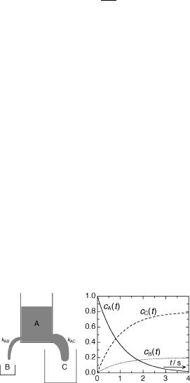
Hence the observed rate constant for the disappearance of A, kobs ¼ kAB þ kAC, is the same as that for the appearance of B (and of C). The difference lies in the pre-exponential partition ratios, kAB/kobs ¼ kAB/(kAB þ kAC) for B, Equation 3.6, and correspondingly kAC/kobs for C, which define the efficiency of the two reactions, as shown in Figure 3.17. Extension of this argument to more than two parallel first-order reactions from a given reactant A is straightforward. The efficiency of a given elementary reaction step is equal to its partition ratio, the rate constant of the process considered, kx, divided by the sum of the rate constants of all processes competing for the depletion the reactant A (Equation 3.7).
hx ¼ kx=Ski
Equation 3.7 Efficiency of a single-step, first-order reaction
Many reaction schemes involving parallel firstand second-order reactions also have straightforward analytical solutions.198 Hence numerical integration methods are rarely required for the fast reactions of interest here. When the reactions are monitored by absorption spectroscopy, the total absorbance of the solution at an observation wavelength l, A(l,t), is related to the concentrations ci of the reacting species Bi by the Beer–Lambert law (Equation 2.5). Thus two parallel reactions, A ! B and C ! D (Scheme 3.1, right) will, in the limit kAB ¼ kCD, give rise to a single exponential obscuring the existence and the relative amplitudes of the two individual steps.
A special problem arises with consecutive reactions, A ! B ! C (Scheme 3.1, centre), that have similar rate constants.199 The integrated rate law for the time-dependent
Figure 3.17 Kinetics of two parallel reactions A ! B and A ! C. Left: illustration with a bucket with two holes of different sizes. Right: concentration profiles of compounds A, B, and C

Flash Photolysis |
101 |
concentration of B is given by Equation 3.8 (concentration profiles for cA to cC are depicted in Figure 3.20). If only B absorbs at the wavelength of observation, then a rise in absorbance will be followed by a decay and it is immediately apparent that a consecutive reaction is being observed. Nonlinear least-squares fitting of an observed kinetic trace using Equation 3.8 will nevertheless be difficult or impossible if kAB kBC, because the expression is indeterminate for kAB ¼ kBC. Moreover, it should be noted that Equation 3.8 is unaffected by an interchange of the microscopic rate constants kAB and kBC, so that the observed rate constants cannot be assigned to the individual steps in the reaction sequence, unless other information, such as the absorption coefficients of intermediates A, B and C, is available. The growth part of a growth–decay curve always corresponds to the faster reaction, but it does not follow that it also corresponds to the first reaction in the sequence.
kAB
cBðtÞ ¼ cAðt ¼ 0Þ kAB kBC ½expð kBCtÞ expð kABtÞ&
Equation 3.8
When the decay of intermediate B is faster than its formation, kBC > kAB, the absolute value of the pre-exponential term will become small and thus the transient concentration cB will be small at all times. For kBC kAB, the appearance of product C will approach the first-order rate law, Equation 3.6 (replace the index B by C), because the transient concentration of intermediate B becomes negligible. This shows that observation of a firstorder rate law for the reaction A ! C does not guarantee that there is no intermediate involved, that is, that the observed reaction A ! C is an elementary reaction.
Rate laws derived for reaction schemes consisting of any number and combination of consecutive, parallel and independent first-order reaction steps can be integrated in closed form to give a sum of exponential terms, so that the total absorbance A of a solution in which these reactions proceed can also be expressed as a sum of exponential terms (Equation 3.9), but see last paragraph of this Section.
AðtÞ ¼ A0 þ A1expð g1tÞ þ A2expð g2tÞ þ
Equation 3.9
First-order decay rate constants of transients that are also subject to second-order reactions cannot be determined reliably, even when attempts are made to correct for the observable second-order contributions. A typical example is the triplet state half-life of anthracene in degassed solution, which appears to be somewhere in the range 20 ms–1 ms on most instruments (the values are reproducible on a given instrument but vary widely between different setups and solvent purification methods). The lifetime of triplet anthracene in solution rises to 25 ms when measures are taken to reduce quenching by diffusional encounters with the parent molecule (self-quenching) with other molecules in the triplet state (triplet–triplet annihilation) and with impurity quenchers such as dioxygen.200 Hence lifetimes of transients that are prone to second-order decay contributions, such as long-lived triplet states or radicals, should always be considered as lower limits.
The response of photomultipliers, photodiodes and diode arrays is generally linear in light flux within a specified range. Within this range, the readings will be proportional to the transmittance T of the sample. Noise associated with the dark current is commonly negligible, because integration times are short. Under these circumstances, the relative

102 |
Techniques and Methods |
error of the transmittance and the absolute error of the sample absorbance, calculated as A ¼ log(1/T), will be constant. Minimization of the squared residuals, x2, with respect to a model function such as Equation 3.9 should therefore be done with absorbance data where each data point properly receives equal weighting. It is not recommended to transform the data points in order to obtain a linear model function, for example, to logA for first-order reactions or to A 1 for second-order reactions, because the associated errors transform accordingly so that weighting of the data points would be required.
Therefore, the trial model function will in general be a nonlinear function of the independent variable, time. Various mathematical procedures are available for iterative x2 minimization of nonlinear functions. The widely used Marquardt procedure is robust and efficient. Not all the parameters in the model function need to be determined by iteration. Any kinetic model function such as Equation 3.9 consists of a mixture of linear parameters, the amplitudes of the absorbance changes, Ai, and nonlinear parameters, the rate constants, ki. For a given set of ki, the linear parameters, Ai can be determined without iteration (as in any linear regression) and they can, therefore, be eliminated from the parameter space in the nonlinear least-squares search. This increases reliability in determining the global minimum and reduces the required computing time considerably.
Although analytical model functions (closed integral forms of the differential kinetic equations) are available for most reaction schemes encountered in fast kinetics, it is by no means trivial in general to derive the physically relevant rate constants ki of the elementary reactions from the observable rate coefficients gi (Equation 3.9) and to determine the concentration profiles from the model parameters gi determined by the fit. Moreover, such a mathematical model will be consistent with many mechanisms (combinations of elementary reactions). In such a situation of mathematical ambiguity, additional information is required. It may consist of mechanistic considerations based on chemical intuition or prior independent knowledge of individual molar absorption coefficients and/ or rate constants. Distinctions between acceptable and unacceptable mechanisms may also be possible on the grounds that the absorbances of all species must be non-negative throughout the spectrum and that the concentrations of all species must be non-negative at all times. As a rule, one should never postulate a mechanism that is more complex than is required by the observed rate law, unless there is other solid evidence requiring a more complex mechanism (Occam s razor).b
3.7.5Global Analysis of Transient Optical Spectra
Recommended textbooks.201,202
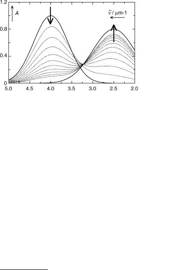
Most absorption and emission spectrophotometers are interfaced to a computer, allowing for digital recording of the spectra. If the spectra change in time, for example when a photoreaction is monitored intermittently by absorption spectroscopy, one obtains a series of spectra such as that shown in Figure 3.18, where the absorbance data are stored in a
b Occam s razor (sometimes spelled Ockham s razor) is a principle attributed to the 14th-century English logician and Franciscan friar William of Ockham. The principle states that the explanation of any phenomenon should make as few assumptions as possible, eliminating those that make no difference in the observable predictions of the explanatory hypothesis or theory. The principle is often expressed in Latin as the lex parsimoniae ( law of parsimony or law of succinctness ): entia non sunt multiplicanda praeter necessitatem, that is, entities should not be multiplied beyond necessity. This is often paraphrased as All other things being equal, the simplest solution is the best. [Quoted from Wikipedia, 14 November 2007.]
Flash Photolysis |
103 |
Figure 3.18 A series of time-dependent spectra
matrixcA (Equation 3.10). Singular value decomposition (SVD) is the method of choice to analyse such data.201 Different names such as principal component analysis and factor analysis are used for essentially the same procedures. These methods are often incorporated in the software provided with the spectrometers. It is important, however, to understand what they do and to what extent they reflect the predilections of the user.
|
0 Aðt2 |
; n~1Þ |
Aðt2 |
; n~2Þ |
. . . Aðt2 |
; n~j Þ |
. . . Aðt2 |
; n~cÞ 1 |
|
|||||||||||
|
A t1 |
; n~1 |
A t1 |
; n~2 |
. . . |
A t1 |
; n~j |
|
. . . |
A t1 |
; n~c |
|
|
|||||||
A ti; n~j |
B ð . . . |
Þ |
ð . . . |
Þ |
. . . |
ð. . . |
Þ |
. . . |
ð . . . |
Þ C |
Aij |
|||||||||
ð Þ ¼ |
B A ti; n~1 |
|
A ti; n~2 |
|
. . . A ti; n~j |
|
. . . A ti; n~c |
|
C |
¼ ð Þ |
||||||||||
B |
|
|
Þ |
ð. . . |
Þ |
. . . |
ð. . . |
Þ |
. . . |
ð. . . |
Þ |
C |
||||||||
|
B ð. . . |
C |
|
|||||||||||||||||
|
B |
|
|
|
|
|
|
|
|
|
|
|
|
|
|
|
|
|
C |
|
|
B A |
tr |
; n~1 |
|
A |
tr |
; n~2 |
|
. . . A |
tr |
; n~j |
|
. . . A |
tr; n~c |
|
C |
|
|||
|
@ ð |
|
|
Þ |
ð |
|
|
Þ |
|
ð |
|
|
Þ |
|
ð |
|
|
Þ A |
|
|
Equation 3.10 Spectral data matrix A of dimension (r c)
The r rows of the matrix, i ¼ 1, . . ., r, represent the absorption spectra of the sample at a given time ti and the c columns, j ¼ 1, . . . , c, collect the absorbances at a given wavenumber
c A matrix A ¼ (Aij) is a (r c) rectangular array of numbers Aij (Equation 3.10); r is the number of rows with index i ¼ 1 r, c the number of columns with index j ¼ 1 c. A square matrix has an equal number of rows and columns, r ¼ c. The transpose A0 of a
matrix A is obtained by exchanging columns and rows, A0 ¼ (Aji). In a diagonal matrix D, all off-diagonal elements vanish, Aij ¼ 0 (i „ j), hence D0 ¼ D. A matrix is symmetrical, if Aji ¼ Aij for all i and j.
Matrix operations are best performed by computer; only some definitions, but not the numerical procedures, are given here. Matrices of equal size (r c) can be added (or subtracted) by adding (or subtracting) their corresponding elements, A B ¼ (Aij Bij). The product C ¼ A B of two matrices can be formed only if the number of columns of A equals the number of rows of B. The elements Cik of C are then given by
m
Cik ¼ P Ail Blk : l¼1
A square matrix is singular if its determinant ||A|| (footnote h at end of Section 1.4) vanishes. The inverse A 1 of a matrix A is defined by the equation A 1 A ¼ E, where E is the identity matrix, E ¼ (dij) and dij is Kronecker s delta, which takes the value of 1 for i ¼ j and 0 otherwise, so that E A ¼ A E ¼ A. The inverse of A can be determined if and only if, it is non-singular, ||A|| „ 0. Diagonalization of a square matrix A is the equivalent of finding its eigenvalues and eigenvectors (Section 1.4).
104 |
Techniques and Methods |
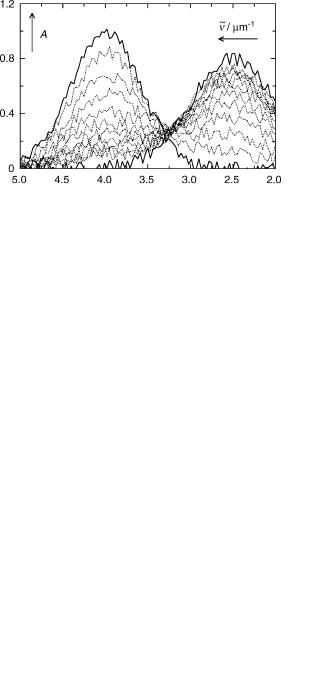
Figure 3.19 Time-dependent spectra of Figure 3.18 with random noise
n~j as a function of time. In the spectra shown, the isosbestic points of consecutive spectra gradually move from 3.3 to 3.2 mm 1, indicating that the overall process observed is not a uniform reaction. The series of spectra was in fact generated artificially assuming a two-step reaction, B1 ! B2 ! B3, with k1 ! 2 ¼ 0.5 s 1 and k2 ! 3 ¼ 2 s 1. Had they been obtained by spectrographic flash photolysis, the signal-to-noise ratio might be around 10 as in Figure 3.19, where random noise was added to the same spectra. In this case, the systematic deviations from a uniform reaction could easily be missed by visual inspection.
According to the Beer–Lambert law (Equation 2.5), the observed absorbances Aij are linear combinations of the absorbances of the three components Bk, k ¼ 1, 2, 3. The matrix A of dimension (r c) was thus constructed by forming the product C «, where the columns of matrix C (r 3) contain the concentration profiles of the species B1–B3 given by the assumed rate law and the rows of matrix « (3 c) contain their spectra (Equation 3.11). To visualize matrix operations, we represent the matrices by rectangles, where the height represents the number of rows and the width the number of columns. For simplicity, the cell length l ¼ 1 cm was multiplied into the matrix elements of «. The concentration profiles and spectra of B1–B3 are plotted in Figure 3.20.
Figure 3.20 Concentration profiles of the components B1–B3 (left) and their absorption spectra (right)