vstatmp_engl

Given are now N observations xi which follow a normal distribution of unknown width σ to be estimated for known mean µ = 5/3. The reason for this

– in principle here arbitrary – choice will become clear below.

The log-likelihood function for our numerical values is presented in Fig. 6.6b. Deriving with respect to the parameter of interest and setting the result equal to zero we find

1 (x − µ)2

0 = σˆ − σˆ3 , q

σˆ = (x − µ)2 .

Again we obtain a well known result. The mean square deviation of the sample values provides an estimate for the width of the normal distribution. This relation is the usual distribution-free estimate of the standard deviation if the expected value is known. The error bounds from the drop of the log-likelihood function by 1/2 become asymmetric. Solving the respective transcendental equation, thereby neglecting higher orders in 1/N, one finds

Example 79. MLE of the mean of a normal distribution with unknown width (case IIa)

The solution of this problem can be taken from Sect. 3.6.11 where we found

P

that t = (x − µ)/s with s2 = (xi − x)2/[N(N − 1)] = v2/(N − 1) follows the Student’s distribution with N − 1 degrees of freedom.

The corresponding log-likelihood is

with the maximum µ = x. It corresponds to the dashed curve in Fig. 6.6a. From the drop of ln L by 1/2 we get now for the standard error squared the expression

δµ2 = (e1/N − 1)v2 .

This becomes for large N, after expanding the exponential function, very similar to the expression for the standard error in case Ia, whereby σ is exchanged by v.

148 6 Parameter Inference I

Example 80. MLE of the width of a normal distribution with unknown mean (case IIb)

Obviously, shifting a normally distributed distribution or a corresponding sample changes the mean value but not the true or the empirical variance v2 = (x − x)2. Thus the empirical variance v2 can only depend on σ and not on µ. Without going into the details of the calculation, we state that Nv2/σ2 follows a χ2 distribution of N − 1 degrees of freedom.

with the log-likelihood

Nv2 ln L(σ) = −(N − 1) ln σ − 2σ2

corresponding to the dashed curve in Fig. 6.6b. (The numerical value of the true value of µ was chosen such that the maxima of the two curves are located at the same value in order to simplify the comparison.) The MLE is

in agreement with our result (3.15). For the asymmetric error limits we find in analogy to example 78

6.5.3 Likelihood Inference for Several Parameters

We can extend our concept easily to several parameters λk which we combine to a vector λ = {λ1, . . . , λK }.

To find the maximum of the likelihood function, we set the partial derivatives

The error interval is now to be replaced by an error volume with its surface defined again by the drop of ln L by 1/2:

We have to assume, that this defines a closed surface in the parameter space, in two dimensions just a closed contour, as shown in the next example.

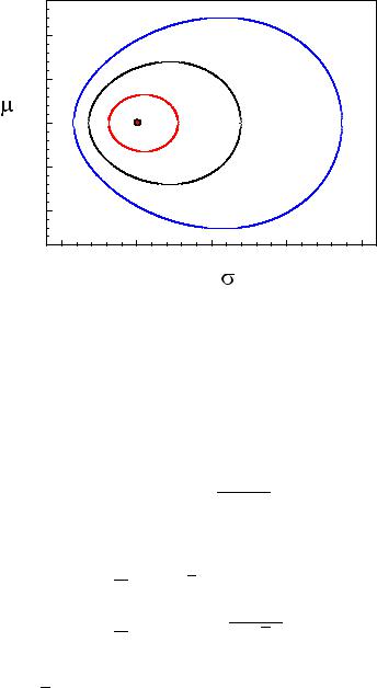
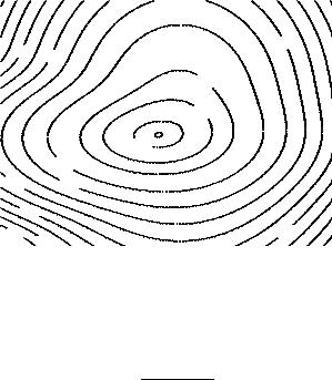
Fig. 6.7. MLE of the parameters of a normal distribution and lines of constant loglikelihood. The numbers indicate the values of log-likelihood relative to the maximum.

Example 81. MLEs of the mean value and the width of a normal distribution

Given are N observations xi which follow a normal distribution where now both the width and the mean value µ are unknown. As above, the loglikelihood is

"#

The derivation with respect to the parameters leads to the results:

1 XN

µˆ = N i=1 xi = x ,

σˆ2 = N1 XN (xi − µˆ)2 = (x − x)2 = v2 .

i=1

The MLE and log-likelihood contours for a sample of 10 events with empirical mean values x = 1 and x2 = 5 are depicted in Fig. 6.7. The innermost line encloses the standard error area. If one of the parameters, for instance µ = µ1 is given, the log-likelihood of the other parameter, here σ, is obtained by the cross section of the likelihood function at µ = µ1.

Similarly any other relation between µ and σ defines a curve in Fig. 6.7 along which a one-dimensional likelihood function is defined.

Remark: Frequently, we are interested only in one of the parameters, and we want to eliminate the others, the nuisance parameters. How to achieve this, will be discussed in Sect. 6.9. Generally, it is not allowed to use the MLE of a single parameter

6.5.4 Combining Measurements

When parameters are determined in independent experiments, we obtain according to the definition of the likelihood the combined likelihood by multiplication of the likelihoods of the individual experiments.

Q

L(λ) = PLi(λ) , ln L = ln Li .

The likelihood method makes it possible to combine experimental results in a extremely simple and at the same time optimal way. Thereby experimental data can originate from completely heterogeneous experiments because no assumptions about the p.d.f.s of the individual experiments enter, except that they are independent of each other.

For the combination of experimental results it is convenient to use the logarithmic presentation. In case the log-likelihoods can be approximated by quadratic parabolas, the addition again produces a parabola.

6.5.5 Normally Distributed Variates and χ2

Frequently we encounter the situation that we have to compare measurements with normally distributed errors to a parameter dependent prediction, for instance when we fit a curve to measurements. (Remark that so far we had considered i.i.d variates, now each observation follows a di erent distribution.) We will come back to this problem below. For the moment let us assume that N observations xi each following a normal distribution with variance δi2

are to be compared to a function ti(θ). The log-likelihood is

The first term of the sum corresponds to the expression (3.6.7) and has been

For parameter inference we can omit the constant terms in (6.13) and thus have

Minimizing χ2 is equivalent to maximizing the log-likelihood. The MLE of θ is obtained from a so-called least square or χ2 fit. Since we obtain the error of the

estimates b from the change of the likelihood function by 1/2, χ2 increases in the

θ

range by one unit, Δχ2 = 1.

152 6 Parameter Inference I

6.5.6 Likelihood of Histograms

For large samples it is more e cient to analyze the data in form of histograms than to compute the likelihood for many single observations. The individual observations are classified and collected into bins where all events of a bin have approximately the same likelihood. We then compare the number of entries of a bin with the parameter dependent prediction. Often the prediction is available only as a Monte Carlo simulation in form of a histogram.

The number of entries di in a bin i follows a multinomial distribution where for each bin the probability pi(θ) is computed as a function of the parameters θ. For a total N of observations the expectation ti of the number of observations in bin i is

ti(θ) = Npi(θ) .

Usually the number of entries of an individual bin is small compared to the total number N. We then are allowed to apply the more comfortable Poisson distribution. The likelihood for ti expected and di observed entries according to the Poisson distribution is given by

ln Li(θ) = −ti + di ln ti − ln(di!) .

Since factors not depending on θ are irrelevant for the likelihood inference (see Sect. 6.5.1), we are allowed to omit the term with the factorial. The log-likelihood of the complete histogram with B bins is then

The parameter dependence is hidden in the quantities ti. The maximum of this function is determined by numerical methods.

For the numerical determination of the maximum, the sum (6.15) has to be recomputed after each modification of the parameters. Since the sum runs only over the bins but not over all individual observations as in the normal likelihood method, the computation for histograms is relatively fast.

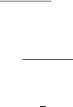
Example 84. Adjustment of a linear distribution to a histogram

The cosine u = cos α of an angle α be linearly distributed according to

f(u|λ) = 12 (1 + λu) , −1 ≤ u ≤ 1 , |λ| < 1 .

We want to determine the parameter λ which best describes the observed distribution of 500 entries di into 20 bins (Fig. 6.8). In the Poisson approximation we expect ti entries for the bin i corresponding to the average value ui = −1 + (i − 0.5)/10 of the cosine,

500

ti = 20 (1 + λui) .

We obtain the likelihood function by inserting this expression into (6.15). The likelihood function an the MLE are indicated in the Figure 6.8.

154 6 Parameter Inference I

= − 12 χ2 .

The sum corresponds to the expression (3.6.7) and has been denoted there as χ2:

χ2 = XB (di − ti)2 .

i=1 ti

If the approximation of the Poisson distribution by a normal distribution is justified, the likelihood estimation of the parameters may be replaced by a χ2 fit and the standard errors are given by a increase of χ2 by one unit.

√

The width of the χ2 distribution for B degrees of freedom is σ = 2B which, for example, is equal to 10 for 50 histogram bins. With such large fluctuations of the value of χ2 from one sample to the other, it appears paradoxical at first sight that a parameter error of one standard deviation corresponds to such a small change of χ2 as one unit, while a variation of χ2 by 10 is compatible with the prediction. The obvious reason for the good resolution is that the large fluctuations from sample to sample are unrelated to the value of the parameter. In case we would compare the prediction after each parameter change to a new measurement sample, we would not be able to obtain a precise result for the estimate of the parameter λ.

Usually, histograms contain some bins with few entries. Then a binned likelihood fit is to be preferred to a χ2 fit, since the above condition of large ti (e.g. ti > 5) is violated. We recommend to perform always a likelihood adjustment.

6.5.7 Extended Likelihood

When we record N independent multi-dimensional observations, {xi} , i = 1, . . . , N, of a distribution depending on a set of parameters θ, then it may happen that these parameters also determine the rate, i.e. the expected rate λ(θ) is a function of θ. In this situation N is no longer an ancillary statistic but a random variable like the xi. This means that we have to multiply two probabilities, the probability to find N observations which follow the Poisson statistics and the probability to observe a certain distribution of the variates xi. Given a p.d.f. f(x|θ) for a single observation, we obtain the likelihood function

Again we can omit the last term in the likelihood analysis, because it does not depend on θ.

As a special case, let us assume that the cross section for a certain reaction is equal to g(x|θ). Then we get the p.d.f. by normalization of g:

x

Fig. 6.9. Likelihood contours.

The production rate λ is equal to the normalization factor multiplied with the luminosity S which is a constant:

Z

λ(θ) = S g(x|θ)dx .

The extended likelihood method is discussed in some detail in Ref. [29].

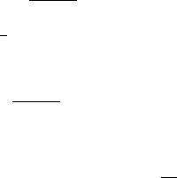
6.5.8 Complicated Likelihood Functions

If the likelihood function deviates considerably from a normal distribution in the vicinity of its maximum, e.g. contains several significant maxima, then it is not appropriate to parametrize it by the maximum and error limits. In this situation the full function or a likelihood map should be presented. Such a map is shown in Fig. 6.9. The presentation reflects very well which combinations of the parameters are supported by the data. Under certain conditions, with more than two parameters, several projections have to be considered.

6.5.9 Comparison of Observations with a Monte Carlo Simulation

Motivation

Modern research in natural sciences requires more and more complex and expensive experimental setups which nevertheless cannot be perfect. Non-linearity, limited acceptance, finite resolution, and dead time a ect the measurements. These e ects can

156 6 Parameter Inference I

be described by an acceptance function α(x, x′) which specifies with which probability a physical quantity x is detected as x′. The acceptance function thus describes at the same time acceptance losses and resolution e ects. A frequency distribution h(x) is convoluted with the acceptance function and transformed to a distribution h′(x′),

XB

Remark that M and thus also cm depends on the parameters which we estimate. Alternatively, we can leave cm as a free parameter in the fit. This is more convenient, but reduces slightly the precision of the estimates of the parameters of interest.

If also the statistical fluctuations of the simulation have to be taken into account and/or the observations are weighted, the expressions for (6.16), (6.17) become more complex. They can be found in Ref. [48], and are for convenience included in Appendix 13.6.

The simulation programs usually consist of two di erent parts. The first part describes the physical process which depends on the parameters of interest. The second models the detection process. Both parts often require large program packages, the so called event generators and the detector simulators. The latter usually consume considerable computing power. Limitations in the available computing time then may result in non-negligible statistical fluctuations of the simulation.