

vstatmp_engl
.pdf3.2 Expected Values |
27 |
|
0.8 |
|
|
g 1 |
= 0 |
||
|
|
|
|
||||
|
0.6 |
|
|
g 2 |
= 17 |
||
f(x) |
g 1 |
= 2 |
|
|
|
|
|
|
|
|
|
|
|
||
|
0.4 |
g 2 |
= 8 |
|
|
|
|
|
|
|
|
g |
1 |
= 0 |
|
|
0.2 |
|
|
g |
2 |
= 2 |
|
|
0.0 |
-5 |
0 |
|
|
|
5 |
|
|
|
|
|
|||
f(x) |
0.1 |
|
|
|
|
|
|
0.01 |
|
|
|
|
|
|
|
1E-3 |
-5 |
0 |
|
|
|
5 |
|
|
|
x |
|
||||
|
|
|
|
|
|
||
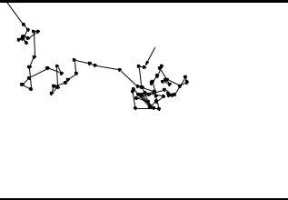
Fig. 3.6. Three distribution with equal mean and variance but di erent skewness and kurtosis.
3.2.6 Discussion
The mean value of a distribution is a so-called position or location parameter, the standard deviation is a scale parameter . A translation of the variate x → y = x + a changes the mean value correspondingly, hyi = hxi + a. This parameter is therefore sensitive to the location of the distribution (like the center of gravity for a mass distribution). The variance (corresponding to the moment of inertia for a mass distribution), respectively the standard deviation remain unchanged. A change of the scale (dilatation) x → y = cx entails, besides hyi = chxi also σ(y) = cσ(x). Skewness and kurtosis remain unchanged under both transformations. They are shape
parameters .
The four parameters mean, variance, skewness, and kurtosis, or equivalently the expected values of x, x2, x3and x4, fix a distribution quite well if in addition the range of the variates and the behavior of the distribution at the limits is given. Then the distribution can be reconstructed quite accurately [74].
Fig. 3.6 shows three probability densities, all with the same mean µ = 0 and standard deviation σ = 1, but di erent skewness and kurtosis. The apparently narrower curve has clearly longer tails, as seen in the lower graph with logarithmic scale.
Mainly in cases, where the type of the distribution is not well known, i.e. for empirical distributions, other location and scale parameters are common. These are the mode xmod, the variate value, at which the distribution has its maximum, and the median, defined as the variate value x0.5, at which P {x < x0.5} = F (x0.5) = 0.5, i.e.
28 3 Probability Distributions and their Properties
the median subdivides the domain of the variate into two regions with equal probability of 50%. More generally, we define a quantile xa of order a by the requirement
F (xa) = a.
A well known example for a median is the half-life t0.5 which is the time at which 50% of the nuclei of an unstable isotope have decayed. From the exponential distribution (3.2) follows the relation between the half-life and the mean lifetime τ
t0.5 = τ ln 2 ≈ 0.693 τ .
The median is invariant under non-linear transformations y = y(x) of the variate,
y0.5 = y(x0.5) while for the mean value µ and the mode xmod this is usually not the case, µy 6= y(µx), ymod 6= y(xmod). The reason for these properties is that probabilities but not probability densities are invariant under variate transformations. Thus
the mode should not be considered as the “most probable value”. The probability to obtain exactly the mode value is zero. To obtain finite probabilities, we have to integrate the p.d.f. over some range of the variate as is the case for the median.
In statistical analyses of data contaminated by background the sample median is more “robust” than the sample mean as estimator of the distribution mean. (see Appendix, Sect. 13.15). Instead of the sample width v, often the full width at half maximum (f.w.h.m.) is used to characterize the spread of a distribution. It ignores the tails of the distribution. This makes sense for empirical distributions, e.g. in the investigation of spectral lines over a sizable background. For a normal distribution the f.w.h.m. is related to the standard deviation by
f.w.h.m.gauss ≈ 2.36 σgauss .
This relation is often used to estimate quickly the standard deviation σ for an empirical distribution given in form of a histogram. As seen from the examples in Fig.3.6, which, for the same variance, di er widely in their f.w.h.m., this procedure may lead to wrong results for non-Gaussian distributions.
3.2.7 Examples
In this section we compute expected values of some quantities for di erent distributions.
Example 11. Expected values, dice
We have p(k) = 1/6, k = 1, . . . , 6.
hxi = (1 + 2 + 3 + 4 + 5 + 6) 1/6 = 7/2 ,
hx2i = (1 + 4 + 9 + 16 + 25 + 36) 1/6 = 91/6 , σ2 = 91/6 − (7/2)2 = 35/12 , σ ≈ 1.71 ,
γ1 = 0 .
The expected value has probability zero.
Example 12. Expected values, lifetime distribution
f(t) = τ1 e−t/τ , t ≥ 0,

htni = Z ∞ tn
0 τ
hV i = |
|
|
|
dr V (r)f(r) |
|||
|
−∞ |
∞ |
|||||
|
4 |
|
|
π |
|||
= |
|
|
√ |
|
|
Z−∞ |
|
3 |
|||||||
|
2πs |
||||||
|
4 |
|
|
π |
∞ |
||
= |
|
|
√ |
|
|
Z−∞ |
|
3 |
|
||||||
|
2πs |
||||||
|
4 |
|
|
π |
∞ |
||
= |
|
|
√ |
|
|
Z−∞ dz (z3 |
|
3 |
|
||||||
|
2πs |
||||||
3.2 Expected Values |
29 |
|
|
|
2 |
+ 3z2r0 |
+ 3zr2 |
+ r3)e− |
z |
2 s2 |
|||
|
0 |
0 |
|
= 43 π(r03 + 3s2r0) .
The mean volume is larger than the volume calculated using the mean radius.
Example 14. Playing poker until the bitter end
Two players are equally clever, but dispose of di erent capital K1, respectively K2 . They play, until one of the players is left without money. We denote the probabilities for player 1, (2) to win finally with w1 (w2). The probability, that one of the two players wins, is unity6:
6That the game ends if the time is not restricted can be proven in game theory and is supported by experience.
30 3 Probability Distributions and their Properties
wall
starting point
wall
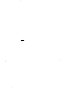
Fig. 3.7. Brownian motion.
w1 + w2 = 1 .
Player 1 gains the capital K2 with probability w1 and looses K1 with probability w2. Thus his mean gain is w1K2 − w2K1. The same is valid for player two, only with reversed sign. As both players play equally well, the expected gain should be zero for both
w1K2 − w2K1 = 0 .
From the two relation follows:
|
K1 |
|
|
K2 |
|
w1 = |
|
; w2 |
= |
|
. |
K1 + K2 |
K1 + K2 |
||||
The probability to win is proportional to the capital disposed of. However, the greater risk of the player with the smaller capital comes along with the possibility of a higher gain.
Example 15. Di usion (random walk)
A particle is moving stochastically according to the Brownian motion, where every step is independent of the previous ones (Fig. 3.7). The starting point has a distance d1 from the wall 1 and d2 from the opposite wall 2. We want to know the probabilities w1, w2 to hit wall 1 or 2. The direct calculation of w1 and w2 is a quite involved problem. However, using the properties of expected values, it can be solved quite simply, without even knowing the probability density. The problem here is completely analogous to the previous one:
|
d2 |
|
|
d1 |
|
w1 = |
|
, |
w2 = |
|
. |
d1 + d2 |
d1 + d2 |
||||
3.2 Expected Values |
31 |
Example 16. Mean kinetic energy of a gas molecule
The velocity of a particle in x-direction vx is given by a normal distribution
1 |
|
|
2 |
2 |
||
f(vx) = |
√ |
|
|
e−vx |
/(2s ) , |
|
|
|
|||||
|
s |
2π |
|
|
||
with |
|
kT |
|
|
||
s2 = |
, |
|
||||
m |
|
|||||
|
|
|
|
|
||
where k, T , m are the Boltzmann constant, the temperature, and the mass of the molecule. The kinetic energy is
ǫkin = m2 (vx2 + vy2 + vz2)
with the expected value
E(ǫkin) = m2 E(vx2 ) + E(vy2) + E(vz2) = 32mE(vx2 ),
where in the last step the velocity distribution was assumed to be isotropic. It follows:
1 |
∞ |
2 |
2 |
||
E(vx2 ) = |
s√ |
|
Z−∞ dvxvx2e−vx |
/(2s ) = s2 = kT/m, |
|
2π |
|||||
3
E(ǫkin) = 2 kT.
Example 17. Reading accuracy of a digital clock
For an accurate digital clock which displays the time in seconds, the deviation of the reading from the true time is maximally ± 0.5 seconds. After the reading, we may associate to the true time a uniform distribution with the actual reading as its central value. To simplify the calculation of the variance, we set the reading equal to zero. We thus have
f(t) = |
1 if − 0.5 < t < 0.5 |
|
|||
|
0 else |
|
|
|
|
and |
0.5 |
1 |
|
|
|
|
|
|
|||
σ2 = Z−0.5 t2 dt = |
. |
(3.16) |
|||
|
|||||
12 |
|||||
The root mean square measurement uncertainty (standard deviation) is σ =
√
1 s/ 12 ≈ 0.29 s.
The variance of a uniform distribution, which covers a range of a, is accordingly σ2 = a2/12. This result is widely used for the error estimation of digital measurements. A typical example from particle physics is the coordinate measurement with a wire chamber.
Example 18. E ciency fluctuations of a detector
A counter registers on average the fraction ε = 0.9 of all traversing electrons. How large is the relative fluctuation σ of the the registered number N1 for N particles passing the detector? The exact solution of this problem requires

32 3 Probability Distributions and their Properties
the knowledge of the probability distribution, in this case the binomial distribution. But also without this knowledge we can derive the dependence on
N with the help of relation (3.13): |
|
√N . |
||
σ |
N1 |
|||
|
N |
|
1 |
|
The whole process can be split into single processes, each being associated
with the passing of a single particle. Averaging over all processes leads to the p
above result. (The binomial distribution gives σ(N1/N) = ε(1 − ε)/N, see Sect. 3.6.1).
All stochastic processes, which can be split into N identical, independent elemen-
√
tary processes, show the typical 1/ N behavior of their relative fluctuations.
3.3 Moments and Characteristic Functions
The characteristic quantities of distributions considered up to now, mean value, variance, skewness, and kurtosis, have been calculated from expected values of the lower four powers of the variate. Now we will investigate the expected value of arbitrary powers of the random variable x for discrete and continuous probability distributions p(x), f(x), respectively. They are called moments of the distribution. Their calculation is particularly simple, if the characteristic function of the distribution is known. The latter is just the Fourier transform of the distribution.
3.3.1 Moments
Definition: The n-th moments of f(x), respectively p(x) are
Z ∞
µn = E(xn) = xnf(x) dx ,
−∞
and
X∞
µn = E(xn) = xnk p(xk)
k=1
where n is a natural number7.
Apart from these moments, called moments about the origin, we consider also the moments about an arbitrary point a where xn is replaced by (x − a)n. Of special importance are the moments about the expected value of the distribution. They are called central moments.
Definition: The n-th central moment about µ = µ1 of f(x), p(x) is:
Z ∞
µ′n = E ((x − µ)n) = (x − µ)nf(x) dx ,
−∞
respectively
7In one dimension the zeroth moment is irrelevant. Formally, it is equal to one.
|
|
|
3.3 Moments and Characteristic Functions |
33 |
||
|
|
|
|
∞ |
|
|
µ′ |
|
− |
µ)n) = |
X |
µ)np(x ) . |
|
= E ((x |
(x |
|
||||
n |
|
|
k − |
k |
|
|
k=1
Accordingly, the first central moment is zero: µ′1 = 0. Generally, the moments are related to the expected values introduced before as follows:
First central moment: µ′1 = 0 Second central moment: µ′2 = σ2 Third central moment: µ′3 = γ1σ3 Fourth central moment: µ′4 = β2σ4
Under conditions usually met in practise, a distribution is uniquely fixed by its moments. This means, if two distributions have the same moments in all orders, they are identical. We will present below plausibility arguments for the validity of this important assertion.
3.3.2 Characteristic Function
We define the characteristic function φ(t) of a distribution as follows: Definition: The characteristic function φ(t) of a probability density f(x) is
|
∞ |
|
φ(t) = E(eitx) = Z−∞ eitxf(x) dx , |
(3.17) |
|
and, respectively for a discrete distribution p(xk) |
|
|
|
∞ |
|
|
X |
|
φ(t) = E(eitx) = |
eitxk p(xk) . |
(3.18) |
k=1
For continuous distributions, φ(t) is the Fourier transform of the p.d.f..
From the definition of the characteristic function follow several useful properties.
φ(t) is a continuous, in general complex-valued function of t, −∞ < t < ∞ with |φ(t)| ≤ 1, φ(0) = 1 and φ(−t) = φ (t). φ(t) is a real function, if and only if the distribution is symmetric, f(x) = f(−x). Especially for continuous distributions there is limt→∞ φ(t) = 0. A linear transformation of the variate x → y = ax + b induces a transformation of the characteristic function of the form
φx(t) → φy (t) = eibtφx(at) . |
(3.19) |
Further properties are found in handbooks on the Fourier transform. The transformation is invertible: With (3.17) it is
∞ |
|
∞ |
∞ |
|
′ |
|
Z−∞ φ(t)e−itx dt = |
Z−∞ e−itx |
Z−∞ eitx |
f(x′) dx′ dt |
|||
|
Z |
∞ |
Z |
∞ |
|
|
= |
|
f(x′) |
|
|
eit(x′−x) dt dx′ |
|
−∞ −∞
Z ∞
= 2π f(x′) δ(x′ − x) dx′
−∞
= 2πf(x) ,

34 3 Probability Distributions and their Properties
f(x) = 1 Z ∞ φ(t)e−itx dt .
2π −∞
The same is true for discrete distributions, as may be verified by substituting (3.18):
|
|
1 |
T |
|
|
|
p(xk) = |
lim |
Z−T φ(t)e− |
itxk |
dt . |
||
|
||||||
|
||||||
T →∞ 2T |
|
|||||
In all cases of practical relevance, the probability distribution is uniquely determined by its characteristic function.
Knowing the characteristic functions simplifies considerably the calculation of moments and of the distributions of sums or linear combinations of variates. For continuous distributions moments are found by n-fold derivation of φ(t):
|
|
nφ(t) |
|
|
|
∞ |
|
|
|
|
||||
|
|
d |
|
|
= |
Z−∞(ix)neitxf(x) dx . |
|
|||||||
|
|
dtn |
|
|
|
|||||||||
With t = 0 follows |
|
|
|
|
∞ |
|
|
|
|
|||||
|
nφ(0) |
|
|
|
|
|
|
|
|
|||||
|
d |
|
= Z−∞(ix)nf(x) dx = inµn . |
(3.20) |
||||||||||
|
dtn |
|||||||||||||
The Taylor expansion of φ(t), |
|
|
|
|
|
|
|
|
|
|
|
|||
|
|
∞ |
|
|
1 |
|
|
dnφ(0) |
∞ |
1 |
|
|
||
|
|
X |
|
|
tn |
|
|
X |
|
(it)nµn , |
(3.21) |
|||
φ(t) = |
|
n! |
dtn |
= |
n=0 |
n! |
||||||||
|
|
n=0 |
|
|
|
|
|
|
|
|
|
|||
generates the moments of the distribution.
The characteristic function φ(t) is closely related to the moment generating function which is defined through M(t) = E(etx). In some textbooks M is used instead of φ for the evaluation of the moments.
We realize that the moments determine φ uniquely, and, since the Fourier transform is uniquely invertible, the moments also determine the probability density, as stated above.
In the same way we obtain the central moments:
Z ∞
φ′(t) = E(eit(x−µ)) = eit(x−µ)f(x) dx = e−itµφ(t) ,
−∞
dnφ′(0) = inµ′ .
dtn n
The Taylor expansion is
φ′(t) = X∞ n1! (it)nµ′n.
n=0
(3.22)
(3.23)
(3.24)
The results (3.20), (3.21), (3.23), (3.24) remain valid also for discrete distributions. The expansion of the right hand side of relation (3.22) allows us to calculate the central moments from the moments about the origin and vice versa:
|
n |
|
µn−kµk |
n |
|
µn′ −kµk . |
|
X |
n |
X |
n |
||
µn′ |
= k=0(−1)k k |
, µn = k=0 k |
||||
Note, that for n = 0 , µ0 = µ′0 = 1.

3.3 Moments and Characteristic Functions |
35 |
In some applications we have to compute the distribution f(z) where z is the sum z = x+ y of two independent random variables x and y with the probability densities g(x) and h(y). The result is given by the convolution integral, see Sect. 3.5.4,
Z Z
f(z) = g(x)h(z − x) dx = h(y)g(z − y) dy
which often is di cult to evaluate analytically. It is simpler in most situations to proceed indirectly via the characteristic functions φg(t), φh(t) and φf (t) of the three p.d.f.s which obey the simple relation
φf (t) = φg(t)φh(t) . |
(3.25) |
Proof:
According to (3.10)we get
φf (t) = E(eit(x+y))
=E(eitxeity)
=E(eitx)E(eity)
=φg(t)φh(t) .
The third step requires the independence of the two variates. Applying the inverse Fourier transform to φf (t), we get
f(z) = |
1 |
Z |
e−itzφf (t) dt . |
2π |
The solution of this integral is not always simple. For some functions it can be found in tables of the Fourier transform.
In the general case where x is a linear combination of independent random variables, x = P cjxj , we find in an analogous way:
Y
φ(t) = φj (cj t) .
Cumulants
As we have seen, the characteristic function simplifies in many cases the calculation of moments and the convolution of two distributions. Interesting relations between the moments of the three distributions g(x), h(y) and f(z) with z = x + y are obtained from the expansion of the logarithm K(t) of the characteristic functions into powers of it:
|
(it)2 |
|
(it)3 |
|
K(t) = ln φ(t) = ln hexp(itx)i = κ1(it) + κ2 |
|
+ κ3 |
|
+ · · · . |
2! |
3! |
|||
Since φ(0) = 1 there is no constant term. The coe cients κi, defined in this way, are called cumulants or semiinvariants. The second notation was chosen, since the cumulants κi, with the exception of κ1, remain invariant under the translations x → x+b of the variate x. Of course, the cumulant of order i can be expressed by moments about the origin or by central moments µk, µ′k up to the order i. We do not present the general analytic expressions for the cummulants which can be derived from the power expansion of exp K(t) and give only the remarkably simple relations for i ≤ 6 as a function of the central moments:

36 3 Probability Distributions and their Properties |
|
||
κ1 = µ1 ≡ µ = hxi , |
|
||
κ2 = µ2′ ≡ σ2 = var(x) , |
|
||
κ3 |
= µ3′ , |
|
|
κ4 = µ4′ |
− 3µ2′ 2 , |
|
|
κ5 = µ5′ |
− 10µ2′ µ3′ , |
(3.26) |
|
κ6 |
= µ6′ |
− 15µ2′ µ4′ − 10µ3′ 2 + 30µ2′ 3 . |
|
Besides expected value and variance, also skewness and excess are easily expressed by cumulants:
γ1 = |
κ3 |
, γ2 = |
κ4 |
. |
(3.27) |
κ3/2 |
|
||||
|
|
κ22 |
|
||
2 |
|
|
|
|
|
Since the product of the characteristic functions φ(t) = φ(1)(t)φ(2)(t) turns into the sum K(t) = K(1)(t)+K(2)(t), the cumulants are additive, κi = κ(1)i +κ(2)iP. In the general case, where x is a linear combination of independent variates, x = cj x(j), the cumulants of the resulting x-distribution, κi, are derived from those of the various x(j) distributions according to
X |
|
κi = cji κi(j) . |
(3.28) |
j
We have met examples for this relation already in Sect. 3.2.3 where we have computed the variance of the distribution of a sum of variates. We will use it again in the discussion of the Poisson distribution in the following example and in Sect. 3.6.3.
3.3.3 Examples
Example 19. Characteristic function of the Poisson distribution
The Poisson distribution
Pλ(k) = λk e−λ k!
has the characteristic function |
|
|
|
|
|
|
φ(t) = |
∞ eitk |
λk |
e−λ |
|||
|
||||||
|
k=0 |
|
k! |
|||
|
X |
|
|
|
||
which can be simplified to |
|
|
|
|
|
|
φ(t) = |
∞ |
1 |
|
(eitλ)ke−λ |
||
|
|
|
||||
|
k! |
|||||
k=0 |
|
|
|
|
|
|
X |
|
|
|
|
|
|
= exp(eitλ)e−λ |
||||||
= exp |
λ(eit − 1) , |
|||||
from which we derive the moments:
dφ = exp λ(eit − 1) λieit , dt
dφ(0) = iλ , dt