

vstatmp_engl
.pdf6.3 Definition and Visualization of the Likelihood |
137 |
6.3 Definition and Visualization of the Likelihood
Usually we do not know the prior or our ideas about it are rather vague.
Example 72. Likelihood ratio: V + A or V − A reaction?
An experiment is performed to measure the energy E of muons produced in the decay of the tau lepton, τ− → µ−ντ ν¯µ, to determine whether the decay corresponds to a V −A or a V +A matrix element. We know the corresponding normalized decay distributions f−(E), f+(E) and we can derive the ratio RL = f−(E)/f+(E). But how should we choose the prior densities for the two alternative hypotheses? In this example it would not make sense to quantify our prejudices for one or the other hypothesis and to publish the resulting probabilities. We restrict the information to the ratio
RL = f−(E) . f+(E)
The quantity RL is called likelihood ratio.
In the absence of prior information the likelihood ratio is the only element which we have, to judge the relative virtues of alternative hypotheses.
Definition: The likelihood Li of a hypothesis Hi, to which corresponds a probability density fi(x) ≡ f(x|Hi) or a discrete probability distribution Wi(k) ≡ P {k|Hi}, when the observation x, k, respectively, has been realized, is equal to
Li ≡ L(i|x) = fi(x)
and
Li ≡ L(i|k) = Wi(k) ,
respectively. Here the index i denoting the hypothesis is treated as an independent random variable. When we replace it by a continuous parameter θ and consider a parameter dependent p.d.f. f(x|θ) or a discrete probability distribution W (k|θ) and observations x, k, the corresponding likelihoods are
L(θ) ≡ L(θ|x) = f(x|θ) ,
L(θ) ≡ L(θ|k) = W (k|θ) .
While the likelihood is related to the validity of a hypothesis given an observation, the p.d.f. is related to the probability to observe a variate for a given hypothesis. In our notation, the quantity which is considered as fixed is placed behind the bar while the variable quantity is located left of it. When both quantities are fixed the function values of both the likelihood and the p.d.f. are equal. To attribute a likelihood makes sense only if alternative hypotheses, either discrete or di ering by parameters, can apply. If the likelihood depends on one or several continuous parameters, we talk of
a likelihood function
Remark: The likelihood function is not a probability density of the parameter. It has no di erential element like dθ involved and does not obey the laws of probability. To distinguish it from probability, R.A. Fisher had invented the name likelihood. Multiplied by a prior and normalized, a probability density of the parameter is obtained. Statisticians call this inverse probability or probability of causes to emphasize
138 6 Parameter Inference I
that compared to the direct probability where the parameter is known and the chances of an event are described, we are in the inverse position where we have observed the event and want to associate probabilities to the various causes that could have led to the observation.
As already stated above, the likelihood of a certain hypothesis is large if the observation is probable for this hypothesis. It measures how strongly a hypothesis is supported by the data. If an observation is very unlikely the validity of the hypothesis is doubtful – however this classification applies only when there is an alternative hypothesis with larger likelihood. Only relations between likelihoods make sense.
Usually experiments provide a sample of N independent observations xi which all follow independently the same p.d.f. f(x|θ) which depends on the unknown parameter
|
˜ |
|
θ (i.i.d. variates). The combined p.d.f. f then is equal to the product of the N simple |
||
p.d.f.s |
|
|
|
|
N |
˜ |
, . . . , xN |θ) = |
f(xi|θ) . |
f(x1 |
||
|
|
=1 |
|
|
iY |
For discrete variates we have the corresponding relation |
||
|
|
N |
˜ |
, . . . , kN |θ) = |
W (ki|θ) . |
W (k1 |
||
|
|
=1 |
|
|
iY |
|
˜ |
evaluated for the sample x1, . . . , xN is equal to the |
|
For all values of θ the function f |
|||
likelihood |
˜ |
|
|
L |
|
|
|
|
˜ |
˜ |
, . . . , xN ) |
|
L(θ) ≡ L(θ|x1,x2 |
||
˜|
=f(x1,x2, . . . , xN θ)
YN
=f(xi|θ)
i=1
YN
=L(θ|xi) .
i=1
The same relation also holds for discrete variates:
˜
L(θ)
≡ ˜ |
L(θ k1, . . . , kN )
YN
=W (ki|θ)
i=1
YN
=L(θ|ki) .
i=1
When we have a sample of independent observations, it is convenient to consider the logarithm of the likelihood. It is called log-likelihood . It is equal to
|
N |
˜ |
Xi |
ln L(θ) = |
ln [f(xi|θ)] |
|
=1 |
for continuous variates. A corresponding relation holds for discrete variates.
6.3 Definition and Visualization of the Likelihood |
139 |
0.8 |
|
|
L=0.00055 |
|
|
y |
|
|
|
|
|
0.6 |
|
|
|
|
|
0.4 |
|
|
|
|
|
0.2 |
|
|
|
|
|
0.0 0 |
1 |
2 |
3 |
4 |
5 |
|
|
|
x |
|
|
L=0.016
0 |
1 |
2 |
3 |
4 |
5 |
|
|
|
x |
|
|
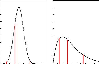
Fig. 6.3. Likelihood of three observations and two hypotheses with di erent p.d.f.s.
Fig. 6.3 illustrates the notion of likelihood in a concrete case of two hypotheses. For two given hypotheses and a sample of three observations we present the values of the likelihood, i.e. the products of the three corresponding p.d.f. values. The broad p.d.f. in the right hand picture matches better. Its likelihood is about thirty times higher than that of the left hand hypothesis.
So far we have considered the likelihood of samples of i.i.d. variates. Also the case where two independent experiments A, B measure the same quantity x is of considerable interest. The combined likelihood L is just the product of the individual
likelihoods LA(θ|x1) = fA(x1|θ) and LB(θ|x2) = fB(x2|θ) as is obvious from the definition:
f(x1, x2|θ) = fA(x1|θ)fB(x2|θ) , L(θ) = f(x1, x2|θ) ,
hence
L = LALB ,
ln L = ln LA + ln LB .
We state: The likelihood of several independent observations or experiments is equal to the product of the individual likelihoods. Correspondingly, the log-likelihoods add up.
Y
L = Li ,
X
ln L = ln Li .
140 6 Parameter Inference I
6.4 The Likelihood Ratio
To discriminate between hypotheses, we use the likelihood ratio. According to a lemma of Neyman and Pearson there is no other more powerful quantity. This means that classifying according to the likelihood ratio, we can obtain the smallest number of false decisions (see Chap. 10). When we have to choose between more than two hypotheses, there are of course several independent ratios.
Example 73. Likelihood ratio of Poisson frequencies
We observe 5 decays and want to compute the relative probabilities for three hypotheses. Prediction H1 assumes a Poisson distribution with expectation value 2, H2 and H3 have expectation values 9 and 20, respectively. The likelihoods following from the Poisson distribution Pλ(k) are:
L1 = P2(5) ≈ 0.036 ,
L2 = P9(5) ≈ 0.061 ,
L3 = P20(5) ≈ 0.00005 .
We can form di erent likelihood ratios. If we are interested for example in hypothesis 2, then the quotient L2/(L1 + L2 + L3) ≈ 0.63 is relevant4. If we observe in a second measurement in the same time interval 8 decays, we obtain:
L1 = P2(5)P2(8) = P4(13) ≈ 6.4 · 10−3 ,
L2 = P9(5)P9(8) = P18(13) ≈ 5.1 · 10−2 ,
L3 = P20(5)P20(8) = P40(13) ≈ 6.1 · 10−7 .
The likelihood ratio L2/(L1 +L2 +L3) ≈ 0.89 (for H1 and H3 correspondingly 0.11 and 10−5) now is much more significant. The fact that all values Li are small is unimportant because one of the three hypotheses has to be valid.
We now apply the same procedure to hypotheses with probability densities.
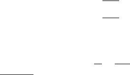
Example 74. Likelihood ratio of normal distributions
We compare samples drawn from one out of two alternative normal distributions with di erent expectation values and variances (Fig. 6.4)
f1 |
= |
√ |
1 |
|
e−(x−1)2/2 , |
|
2π1 |
||||||
|
|
|
|
|||
f2 |
= |
√ |
1 |
|
e−(x−2)2/8 . |
|
2π2 |
||||||
|
|
|
|
|||
a) Initially the sample consists of a single observation at x = 0, for both cases one standard deviation o the mean values of the two distributions (Fig. 6.4a):
L1 = 2 e−1/2 = 2 .
L2 e−4/8
4We remember that the likelihood ratio is not the ratio of the probabilities. The latter depends on prior probabilities of the hypotheses.
6.4 The Likelihood Ratio |
141 |
0.4 |
a) |
|
|
L |
/L |
= 2 |
|
|
|
|
|
1 |
2 |
|
|
f(x) |
|
|
|
|
|
|
|
0.2 |
|
|
|
|
|
|
|
0.0 |
|
|
|
|
|
|
|
0.4 |
c) |
|
|
L |
/L = 30 |
||
|
|
|
1 |
|
2 |
|
|
f(x) |
|
|
|
|
|
|
|
0.2 |
|
|
|
|
|
|
|
0.0-4 |
-2 |
0 |
2 |
4 |
|
6 |
|
|
|
|
x |
|
|
|
|
|
0.4 |
b) |
|
|
|
L |
/L |
= 1.2 |
|
|
|
|
|
|
1 |
2 |
|
|
|
|
0.2 |
|
|
|
|
|
|
|
|
|
0.0 |
|
|
|
|
|
|
|
|
|
0.4 |
d) |
|
|
L |
/L |
= 1/430 |
|
|
|
|
|
1 |
2 |
|
|
|
||
|
0.2 |
|
|
|
|
|
|
|
|
8 |
0.0-4 |
-2 |
0 |
2 |
4 |
|
|
6 |
8 |
|
|
|
|
x |
|
|
|
|
|
Fig. 6.4. Likelihood ratio for two normal distributions. Top: 1 observation, bottom: 5 observations.
b) Now we place the observation at x = 2, the maximum of the second distribution (Fig. 6.4b):
L1 = 2 e−1/2 = 1.2 .
L2 e−0
c) We now consider five observations which have been taken from distribution f1 (Fig. 6.4c) and distribution f2, respectively (Fig. 6.4d). We obtain the likelihood ratios
L1/L2 |
= 30 |
(Fig. 5.3c) , |
L1/L2 |
= 1/430 (Fig. 5.3d) . |
|
It turns out that small distributions are easier to exclude than broad ones. On the other hand we get in case b) a preference for distribution 1 even though the observation is located right at the center of distribution 2.
Example 75. Likelihood ratio for two decay time distributions
A sample of N decay times ti has been recorded in the time interval tmin < t < tmax. The times are expected to follow either an exponential distribution f1(t) e−t/τ (hypothesis 1), or an uniform distribution f2(t) = const. (hypothesis 2). How likely are H1, H2? First we have to normalize the p.d.f.s:

142 |
6 Parameter Inference I |
|
|
|
|
|
|
f1(t) = |
1 |
|
e−t/τ |
||
|
|
|
|
|
, |
|
|
τ |
e−tmin/τ − e−tmax/τ |
||||
|
f2(t) = |
|
1 |
. |
||
|
tmax − tmin |
|||||
The likelihoods are equal to the product of the p.d.f.s at the observations:
L1 |
= |
h |
|
i |
− |
i=1 |
ti/τ! |
, |
τ |
e−tmin/τ − e−tmax/τ |
−N exp |
N |
|||||
L2 |
= |
1/(tmax − tmin)N . |
|
|
X |
|
|
|
|
|
|
|
|
||||
P
With t = ti/N the mean value of the times, we obtain the likelihood ratio
L1 |
= |
tmax |
tmin |
|
N |
||
|
|
|
|||||
|
τ(e−tmin/τ |
− |
e−Nt/τ . |
||||
L2 |
e−tmax/τ ) |
||||||
|
|
|
− |
|
|
|
|
6.5 The Maximum Likelihood Method for Parameter Inference
In the previous examples we have compared a sample with di erent hypotheses which di ered only in the value of a parameter but corresponded to the same distribution. We now allow for an infinite number of hypotheses by varying the value of a parameter. As in the discrete case, in the absence of a given prior probability, the only
available piece of information which allows us to judge di erent parameter values is the likelihood function. A formal justification for this assertion is given by the likelihood principle (LP) which states that the likelihood function exhausts all the information contained in the observations related to the parameters and which we will discuss in the following chapter. It is then plausible to choose the parameter such that the likelihood is as large as possible. This is the maximum likelihood estimate (MLE). When we are interested in a parameter range, we will choose the interval such that the likelihood outside is always less than inside.
Remark that the MLE as well as likelihood intervals are invariant against transformations of the parameter. The likelihood is not a p.d.f. but a function of the parameter and therefore L(θ) = L′(θ′) for θ′(θ). Thus a likelihood analysis estimating, for example, the mass of a particle will give the same result as that inferring the mass squared, and estimates of the decay rate γ and mean life τ = 1/γ will be consistent.
Here and in the following sections we assume that the likelihood function is continuous and di erentiable and has exactly one maximum inside the valid range of the parameter. This condition is fulfilled in the majority of all cases.
Besides the maximum likelihood (ML) method, invented by Fisher, there exist a number of other methods of parameter estimation. Popular is especially the method of least squares (LS) which was first proposed by Gauß5. It is used to adjust parameters of curves which are fixed by some measured points and will be discussed in the next chapter. It can be traced back to the ML method if the measurement errors are normally distributed.
5Carl Friedrich Gauß (1777-1855), German mathematician, astronomer and physicist.
6.5 The Maximum Likelihood Method for Parameter Inference |
143 |
0.5 |
2.0 |
4.5 |
ln(L) |
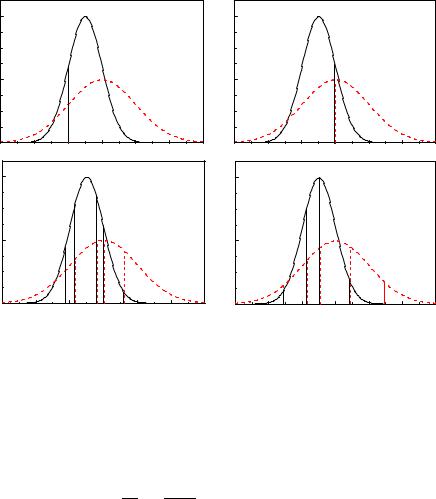
Fig. 6.5. Log-likelihood function and uncertainty limits for 1, 2, 3 standard deviations.
In most cases we are not able to compute analytically the location of the maximum of the likelihood. To simplify the numerical computation, still linear approximations (e.g. linear regression) are used quite frequently. These methods find the solution by matrix operations and iteration. They are dispensable nowadays. With common PCs and maximum searching programs the maximum of a function of some hundred parameters can determined without problem, given enough observations to fix it.
6.5.1 The Recipe for a Single Parameter
We proceed according to the following recipe. Given a sample of N i.i.d. observations {x1, . . . , xN } from a p.d.f. f(x|θ) with unknown parameter θ, we form the likelihood or its logarithm, respectively, in the following way:
|
|
N |
|
|
(6.6) |
L(θ) = |
i=1 f(xi|θ) , |
||||
|
P |
N |
| |
|
(6.7) |
ln L(θ) = |
Qi=1 ln f(xi |
θ) . |
|||

144 6 Parameter Inference I
In most cases the likelihood function resembles a bell shaped Gaussian and ln L(θ) approximately a downwards open parabola (see Fig. 6.5). This approximation is especially good for large samples.
To find the maximum of L (ln L and L have their maxima at the same location), we derive the log-likelihood6 with respect to the parameter and set the derivative
equal to zero. The value ˆ, that satisfies the equation which we obtain in this way is
θ
the MLE of θ.
d ln L |
|θˆ = 0 |
(6.8) |
dθ |
Since only the derivative of the likelihood function is of importance, factors in the likelihood or summands in the log-likelhood which are independent of θ can be omitted.
The estimate ˆ is a function of the sample values , and consequently a statistic.
θ xi
The point estimate has to be accompanied by an error interval. Point estimate and error interval form an ensemble and cannot be discussed separately. Choosing as point estimate the value that maximizes the likelihood function it is natural to include inside the error limits parameter values with higher likelihood than all parameters that are excluded. This prescription leads to so-called likelihood ratio error intervals.
We will discuss the error interval estimation in a separate chapter, but fix the error limit already now by definition:
Definition: The limits of a standard error interval are located at the parameter values where the likelihood function has decreased from its maximum by a factor e1/2. For two and three standard deviations the factors are e2 and e4.5. This choice corresponds to di erences for the log-likelihood of 0.5 for one, of 2 for two and of 4.5 for three standard error intervals as illustrated in Fig. 6.5. For the time being we assume that these limits exist inside the parameter range.
The reason for this definition is the following: As already mentioned, asymptotically, when the sample size N tends to infinity, under very general conditions the likelihood function approaches a Gaussian and becomes proportional to the probability density of the parameter (for a proof, see Appendix 13.3). Then our error limit corresponds exactly to the standard deviation of the p.d.f., i.e. the square root of the variance of the Gaussian. We keep the definition also for non normally shaped likelihood functions and small sample sizes. Then we usually get asymmetric error limits.
6.5.2 Examples
Example 76. Maximum likelihood estimate (MLE) of the mean life of an unstable particle
Given be N decay times ti of an unstable particle with unknown mean life τ. For an exponential decay time distribution
f(t|γ) = γe−γt
with γ = 1/τ the likelihood is
6The advantage of using the log-likelihood compared to the normal likelihood is that we do not need to derive a product but a sum which is much more convenient.

6.5 The Maximum Likelihood Method for Parameter Inference |
145 |
|
|
|
|
|
N |
|
|
|
|
|
L = γN |
e−γti |
|||||
|
|
|
|
|
=1 |
|
|
|
|
|
|
|
|
iY |
|
|
|
|
|
|
|
|
N |
γt |
||
|
|
|
|
|
|
|||
|
|
= γN e− Pi=1 Ni , |
||||||
|
ln L = N ln γ − γ |
ti . |
||||||
|
|
|
|
|
|
=1 |
|
|
The estimate γˆ satisfies |
|
|
|
|
Xi |
|||
|
|
|
|
|
|
|
||
|
d ln L |
|γˆ = 0 , |
|
|
|
|
||
|
|
|
|
|
|
|||
|
dγ |
|
|
|
|
|||
|
|
|
|
|
N |
|
|
|
|
|
|
N |
Xi |
|
|
|
|
|
|
0 = |
γˆ |
|
− ti , |
|||
|
|
|
|
|
=1 |
|
|
|
|
|
|
|
|
N |
|
|
|
|
|
|
|
|
Xi |
|
|
|
|
|
τˆ = γˆ−1 = |
ti/N = |
t |
. |
|||
|
|
|
|
|
=1 |
|
|
|
Thus the estimate is just equal to the mean value t of the observed decay times. In practice, the full range up to infinitely large decay times is not always observable. If the measurement is restricted to an interval 0 < t < tmax, the p.d.f. changes, it has to be renormalized:
f(t|γ) = |
|
γe−γt |
|
, |
|
|||
1 |
− |
e |
− |
γtmax |
|
|||
|
|
|
|
|
|
|
||
|
|
|
|
|
|
|
|
N |
|
|
|
|
|
|
Xi |
||
ln L = N ln γ − ln(1 − e−γtmax ) |
− γ |
ti . |
||||||
|
|
|
|
|
|
|
|
=1 |
The maximum is now located at the estimate γˆ, which fulfils the relation
0 = N |
|
|
− |
N |
1 |
|
X |
||
|
t e−γtˆ max |
− i=1 ti , |
||
|
− |
max |
||
γˆ |
1 e−γtˆ max |
τˆ = |
|
+ |
tmaxe−tmax/τˆ |
, |
|
t |
|||||
1 − e−tmax/τˆ |
|||||
|
|
|
|
which has to be evaluated numerically. If the time interval is not too short, tmax > τ, an iterative computation lends itself: The correction term at the right hand side is neglected in zeroth order. At the subsequent iterations we insert in this term the value τ of the previous iteration. We notice that the estimate again depends solely on the mean value t of the observed decay times. The quantity t is a su cient statistic. We will explain this notion in more detail later. The case with also a lower bound tmin of t can be reduced easily to the previous one by transforming the variable to t′ = t − tmin.
In the following examples we discuss the likelihood functions and the MLEs of the parameters of the normal distribution in four di erent situations:
Example 77. MLE of the mean value of a normal distribution with known width (case Ia)
Given are N observation xi drawn from a normal distribution of known width σ and mean value µ to be estimated:
146 |
6 |
Parameter Inference I |
|
||
|
|
0.0 |
a) |
|
|
|
|
|
|
|
|
|
|
-0.5 |
|
|
|
|
|
lnL |
|
|
|
|
|
-1.0 |
|
|
|
|
|
-1.5 |
|
|
|
|
|
-2.0 |
0 |
1 |
2 |
|
|
|
|||
0.0 |
b) |
|
|
|
|
|
|
-0.5 |
|
|
|
-1.0 |
|
|
|
-1.5 |
|
|
|
-2.0 1 |
2 |
3 |
4 |
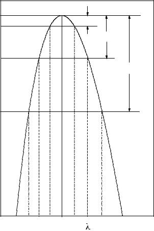
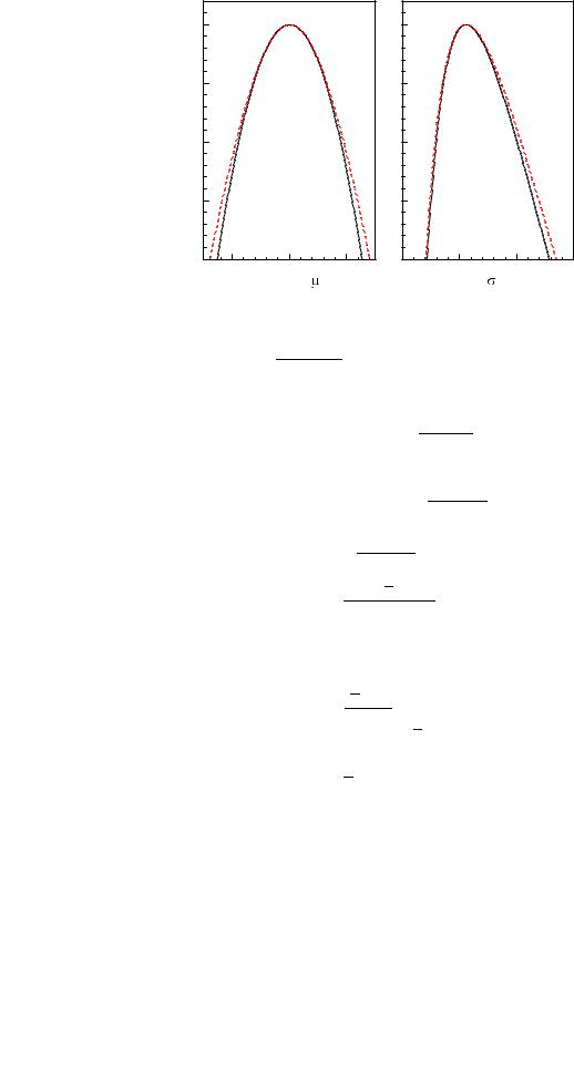
Fig. 6.6. Log-likelihood functions for the parameters of a normal distribution: a) for the mean µ with known width (solid curve) and unknown width (dashed curve), b) for the
width σ with known mean (solid curve) and unknown mean (dashed curve). The position p
of the maximum is σˆ = σ N/(N − 1) = 2.108 for both curves.
| |
|
√2πσ |
|
− |
|
|
2σ2 |
|
|
|||||
f(x µ) = |
1 |
|
|
exp |
(x − µ)2 |
|
, |
|||||||
|
|
|
|
|
|
|
|
|||||||
|
N |
|
|
|
|
|
|
|
|
|
|
|||
L(µ) = |
Y |
1 |
|
exp |
|
(xi − µ)2 |
, |
|||||||
|
|
|
|
|
|
|
|
|
|
|||||
|
i=1 √2πσ |
|
− |
|
2σ2 |
|
|
|||||||
|
|
Xi |
|
|
|
|
|
|
|
|
|
|
||
ln L(µ) = |
− |
N |
(xi |
− µ)2 |
+ const |
|
(6.9) |
|||||||
=1 |
|
|
2σ2 |
|
||||||||||
|
|
|
|
|
|
|
|
|||||||
|
|
|
|
|
|
|
|
|
|
|
|
|||
|
|
|
xµ + µ2 |
|
||||||||||
= |
− |
N |
x2 |
− 2 |
+ const . |
|||||||||
|
|
|
|
|
||||||||||
|
|
|
|
|
|
|
2σ2 |
|
|
|
|
|
||
The log-likelihood function is a parabola. It is shown in Fig. 6.6a for σ = 2. Deriving it with respect to the unknown parameter µ and setting the result equal to zero, we get
N (x − µˆ) = 0 , σ2
µˆ = x .
The likelihood estimate µˆ for the expectation value of the normal distribution is equal to the arithmetic mean x of the sample. It is independent of σ, but
σ determines the width of the likelihood function and the standard error
√
δµ = σ/ N.
Example 78. MLE of the width of a normal distribution with given mean (case Ib)