vstatmp_engl

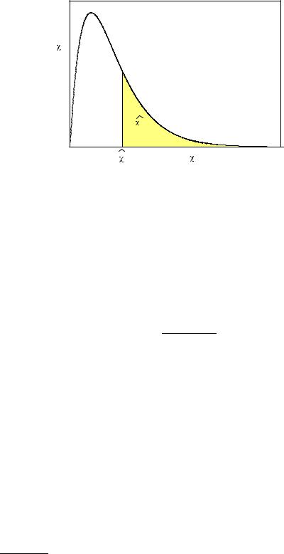
When we test, for instance, the hypothesis that a coordinate is distributed according to N(0, 1), then for a sample consisting of a single measurement x, a reasonable test statistic is the absolute value |x|. We assume that if H0 is wrong then |x| would be large. A typical test statistic is the χ2 deviation of a histogram from a prediction. Large values of χ2 indicate that something might be wrong with the prediction.

Before we apply the test we have to fix a critical region K which leads to the rejection of H0 if t is located inside of it. Under the condition that H0 is true, the probability of rejecting H0 is α, P {t K|H0} = α where α [0, 1] normally is a small quantity (e.g. 5 %). It is called significance level or size of the test. For a test

based on the χ2 statistic, the critical region is defined by χ2 > χ2max(α) where the parameter χ2max is a function of the significance level α. It fixes the range of the

critical region.

To compute rejection probabilities we have to compute the p.d.f. f(t) of the test statistic. In some cases it is known as we will see below, but in other cases it has to be obtained by Monte Carlo simulation. The distribution f has to include all experimental conditions under which t is determined, e.g. the measurement uncertainties of t.

10.2.3 Errors of the First and Second Kind, Power of a Test

After the test parameters are selected, we can apply the test to our data. If the actually obtained value of t is outside the critical region, t / K, then we accept H0, otherwise we reject it. This procedure implies four di erent outcomes with the following a priori probabilities:

1. H0 ∩ t K, P {t K|H0} = α: error of the first kind. (H0 is true but rejected.),

2.H0 ∩ t / K, P {t / K|H0} = 1 − α (H0 is true and accepted.),

3.H1 ∩ t K, P {t K|H1} = 1 − β (H0 is false and rejected.),

4.H1 ∩ t / K, P {t / K|H1} = β: error of the second kind (H0 is false but accepted.).

When we apply the test to a large number of data sets or events, then the rate α, the error of the first kind, is the ine ciency in the selection of H0 events, while the rate β, the error of the second kind, represents the background with which the selected events are contaminated with H1 events. Of course, for α given, we would like to have β as small as possible. Given the rejection region K which depends on α, also β is fixed for given H1. For a reasonable test we expect that β is monotonically decreasing with α increasing: With α → 0 also the critical region K is shrinking, while the power 1 − β must decrease, and the background is less suppressed. For fixed α, the power indicates the quality of a test, i.e. how well alternatives to H0 can be rejected.

The power is a function, the power function, of the significance level α. Tests which provide maximum power 1 − β with respect to H1 for all values of α are called Uniformly Most Powerful (UMP) tests. Only in rare cases where H1 is restricted in some way, there exists an optimum, i.e. UMP test. If both hypotheses are simple then as already mentioned in Chap. 6, Sect. 6.3, according to a lemma of Neyman and E. S. Pearson, the likelihood ratio can be used as test statistic to discriminate between H0 and H1 and provides a uniformly most powerful test.

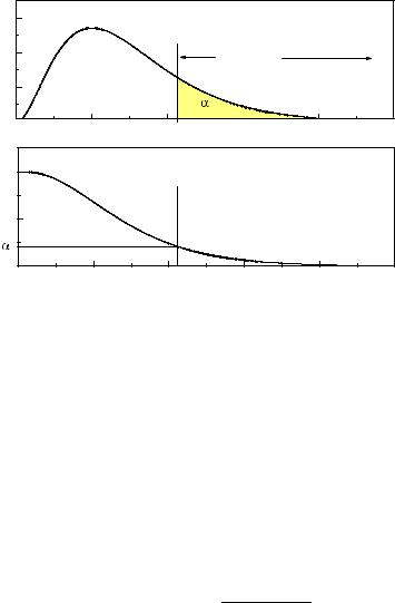
Fig. 10.1. Distribution of a test statistic and corresponding p-value curve.

When H1 represents a family of distributions, consistency and non-biasedness are valid only if they apply to all members of the family. Thus in case that the alternative H1 is not specified, a test is biased if there is an arbitrary hypothesis di erent from H0 with rejection probability less than α and it is inconsistent if we can find a hypothesis di erent from H0 which is not rejected with power unity in the large sample limit.

Example 125. Bias and inconsistency of a test

Assume, we select in an experiment events of the type K0 → π+π−. The invariant mass mππ of the pion pairs has to match the K0 mass. Due to the finite experimental resolution the experimental masses of the pairs are normally distributed around the kaon mass mK with variance σ2. With the null hypothesis H0 that we observe K0 → π+π− decays, we may apply to our sample a test with the test quantity t = (mππ − mK )2/σ2, the normalized mean quadratic di erence between the observed masses of N pairs and the nominal K0 mass. Our sample is accepted if it satisfies t < t0 where t0 is the critical quantity which determines the error of the first kind α and the acceptance 1 − α. The distribution of Nt under H0 is a χ2 distribution with N degrees of freedom. Clearly, the test is biased, because we can imagine mass distributions with acceptance larger than 1 − α, for instance a uniform distribution in the range t ≤ t0. This test is also inconsistent, because it would favor this specific realization of H1 also for infinitely large samples. Nevertheless it is not unreasonable for very small samples in the considered case and for N = 1 there is no alternative. The situation is di erent for large samples where more powerful tests exist which take into account the Gaussian shape of the expected distribution under H0.

250 10 Hypothesis Tests

While consistency is a necessary condition for a sensible test applied to a large sample, bias and inconsistency of a test applied to a small sample cannot always be avoided and are tolerable under certain circumstances.

10.3 Goodness-of-Fit Tests

10.3.1 General Remarks

Goodness-of-fit (GOF) tests check whether a sample is compatible with a given distribution. Even though this is not possible in principle without a well defined alternative, this works quite well in practice, the reason being that the choice of the test statistic is influenced by speculations about the behavior of alternatives, speculations which are based on our experience. Our presumptions depend on the specific problem to be solved and therefore very di erent testing procedures are on the market.

In the empirical research outside the exact sciences, questions like “Is a certain drogue e ective?”, “Have girls less mathematical ability than boys?”, “Does the IQ follow a normal distribution? ” are to be answered. In the natural sciences, GOF tests usually serve to detect unknown systematic errors in experimental results. When we measure the mean life of an unstable particle, we know that the lifetime distribution is exponential but to apply a GOF test is informative, because a low p-value may indicate a contamination of the events by background or problems with the experimental equipment. But there are also situations where we accept or reject hypotheses as a result of a test. Examples are event selection (e.g. B-quark production), particle track selection on the bases of the quality of reconstruction and particle identification, (e.g. electron identification based on calorimeter or Cerenkov information). Typical for these examples is that we examine a number of similar objects and accept a certain error rate α, while when we consider the p-value of the final result of an experiment, discussing an error rate does not make sense.

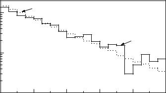
An experienced scientist has a quite good feeling for deviations between two distributions just by looking at a plot. For instance, when we examine the statistical distribution of Fig. 10.2, we will realize that its description by an exponential distribution is rather unsatisfactory. The question is: How can we quantify the disagreement? Without a concrete alternative it is rather di cult to make a judgement.

Let us discuss a di erent example: Throwing a dice produces “1” ten times in sequence. Is this result compatible with the assumption H0 that the dice is unbiased? Well, such a sequence does not occur frequently and the guess that something is wrong with the dice is well justified. On the other hand, the sequence of ten times “1” is not less probable than any other sequence, namely (1/6)10 = 1. 7 · 10−8. Our doubt relies on our experience: We have an alternative to H0 in mind, namely asymmetric dice. We can imagine asymmetric dice but not dice that produce with high probability a sequence like “4,5,1,6,3,3,6,2,5,2”. As a consequence we would choose a test which is sensitive to deviations from a uniform distribution. When we test a random number generator we would be interested, for example, in a periodicity of the results or a correlation between subsequent numbers and we would choose a di erent test. In GOF tests, we cannot specify H1 precisely, but we need to have an idea of it which then enters in the selection of the test. We search for test parameters where we suppose that they discriminate between the null hypothesis and possible alternatives.

Fig. 10.2. Comparison of an experimental distribution to a prediction.

However, there is not such a thing as a best test quantity as long as the alternative is not completely specified.

A typical test quantity is the χ2-variable which we have introduced to adjust parameters of functions to experimental histograms or measured points with known error distributions. In the least square method of parameter inference, see Chap. 7, the parameters are fixed such that the sum χ2 of the normalized quadratic deviations is minimum. Deviating parameter values produce larger values of χ2, consequently we expect the same e ect when we compare the data to a wrong hypothesis. If χ2 is abnormally large, it is likely that the null hypothesis is not correct.

Unfortunately, physicists use almost exclusively the χ2 test, even though for many applications more powerful tests are available. Scientists also often overestimate the significance of the χ2 test results. Other tests like the Kolmogorov–Smirnov Test and tests of the Cramer–von Mises family avoid the always somewhat arbitrary binning of histograms in the χ2 test. These tests are restricted to univariate distributions, however. Other binning-free methods can also be applied to multivariate distributions.

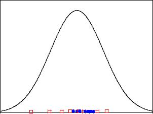
Sometimes students think that a good test statistic would be the likelihood L0 of the null hypothesis, i.e. for H0 with single event distribution f0(x) the product Πf0(xi). That this is not a good idea is illustrated in Fig. 10.3 where the null hypothesis is represented by a fully specified normal distribution. From the two samples, the narrow one clearly fits the distribution worse but it has the higher likelihood. A sample where all observations are located at the center would per definition maximize the likelihood but such a sample would certainly not support the null hypothesis.

While the indicated methods are distribution-free, i.e. applicable to arbitrary distributions specified by H0, there are procedures to check the agreement of data with specific distributions like normal, uniform or exponential distributions. These methods are of inferior importance for physics applications. We will deal only with distribution-free methods.

252 10 Hypothesis Tests

Fig. 10.3. Two di erent samples and a hypothesis.

We will also exclude tests based on order statistics from our discussion. These tests are mainly used to test properties of time series and are not very powerful in most of our applications.

At the end of this section we want to stress that parameter inference with a valid hypothesis and GOF test which doubt the validity of a hypothesis touch two completely di erent problems. Whenever possible deviations can be parameterized it is always appropriate to determine the likelihood function of the parameter and use the likelihood ratio to discriminate between di erent parameter values.

A good review of GOF tests can be found in [57], in which, however, more recent developments are missing.

10.3.2 P-Values

Interpretation and Use of P-Values

We have introduced p-values p in order to dispose of a quantity which measures the agreement between a sample and a distribution f0(t) of the test statistic t. Small p-values should indicate a bad agreement. Since the distribution of p under H0 is uniform in the interval [0, 1], all values of p in this interval are equally probable. When we reject a hypothesis under the condition p < 0.1 we have a probability of 10% to reject H0. The rejection probability would be the same for a rejection region p > 0.9. The reason for cutting at low p-values is the expectation that distributions of H1 would produce low p-values.

The p-value is not the probability that the hypothesis under test is true. It is the probability under H0 to obtain a p-value which is smaller than the one actually observed. A p-value between zero and p is expected to occur in the fraction p of experiments if H0 is true.

Fig. 10.4. Comparison of two experimental histograms to a uniform distribution.

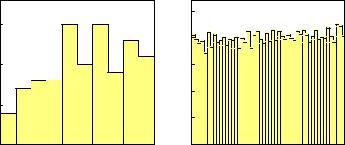
Example 126. The p-value and the probability of a hypothesis

In Fig. 10.4 we have histogrammed two distributions from two simulated experiments A and B. Are these uniform distributions? For experiment B with 10000 observations this is conceivable, while for experiment A with only 100 observations it is di cult to guess the shape of the distribution. Alternatives like strongly rising distributions are more strongly excluded in B than in A. We would therefore attribute a higher probability for the validity of the hypothesis of a uniform distribution for B than for A, but the p-values based on the χ2 test are very similar in both cases, namely p ≈ 0.08. Thus the deviations from a uniform distribution would have in both cases the same significance

We learn from this example also that the p-value is more sensitive to deviations in large samples than in small samples. Since in practice small unknown systematic errors can rarely be excluded, we should not be astonished that in high statistics experiments often small p-values occur. The systematic uncertainties which usually are not considered in the null hypothesis then dominate the purely statistical fluctuation.

Even though we cannot transform significant deviations into probabilities for the validity of a hypothesis, they provide useful hints for hidden measurement errors or contamination with background. In our example a linearly rising distribution has been added to uniform distributions. The fractions were 45% in experiment A and 5% in experiment B.

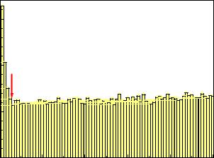
In some experimental situations we are able to compare many replicates of measurements to the same hypothesis. In particle physics experiments usually a huge number of tracks has to be reconstructed. The track parameters are adjusted by a χ2 fit to measured points assuming normally distributed uncertainties. The χ2 value of each fit can be used as a test statistic and transformed into a p-value, often called χ2 probability. Histograms of p-values obtained in such a way are very instructive. They often look like the one shown in Fig. 10.5. The plot has two interesting features: It is slightly rising with increasing p-value which indicates that the errors have been slightly overestimated. The peak at low p-values is due to fake tracks which do not correspond to particle trajectories and which we would eliminate almost completely by a cut at about pc = 0.05. We would have to pay for it by a loss of good tracks of

Z

pk = f0(x) dx ,

k

with Σpk = 1. The integration extends over the interval k. The number of sample observations dk found in this bin has to be compared with the expectation value Npk. To interpret the deviation dk − Npk, we have to evaluate the expected mean quadratic deviation δk2 under the condition that the prediction is correct. Since the distribution of the observations into bins follows a binomial distribution, we have

δk2 = Npk(1 − pk) .

Usually the observations are distributed into typically 10 to 50 bins. Thus the probabilities pk are small compared to unity and the expression in brackets can be omitted. This is the Poisson approximation of the binomial distribution. The mean quadratic deviation is equal to the number of expected observations in the bin:

δk2 = Npk .

We now normalize the observed to the expected mean quadratic deviation,

k=1 Npk

By construction we have:

hχ2ki ≈ 1 , hχ2i ≈ B .

If the quantity χ2 is considerably larger than the number of bins, then obviously the measurement deviates significantly from the prediction.

A significant deviation to small values χ2 B even though considered as unlikely is tolerated, because we know that alternative hypotheses do not produce smaller hχ2i than H0.

The χ2 Distribution and the χ2 Test

We now want to be more quantitative. If H0 is valid, the distribution of χ2 follows to a very good approximation the χ2 distribution which we have introduced in Sect. 3.6.7 and which is displayed in Fig. 3.20. The approximation relies on the approximation of the distribution of observations per bin by a normal distribution, a condition which in most applications is su ciently good if the expected number of entries per bin is larger than about 10. The parameter number of degrees of freedom (NDF ) f of the χ2 distribution is equal to the expectation value and to the number of bins minus one: