vstatmp_engl

χ2 = χ2stat + Rregu , ln L = ln Lstat − Rregu .

This term is constructed in such a way that smooth functions are favored. It has to get larger for stronger fluctuations of the solution.

3.The deconvolution is performed iteratively, starting from a smooth zeroth approximation of the true distribution. The iteration is stopped, once insignificant oscillations appear.

4.Insignificant eigenvalues of the transfer matrix are suppressed.

Of course, the size of the regularization must be limited such that the deconvoluted function is still compatible with the observation. This condition is used to fix the regularization parameter.

We will restrict our considerations to the methods 2 to 4. The accuracy of method 1 is hard to estimate. Reviews and comparisons of some deconvolution methods can be found in [47, 48, 50, 51, 52].

9.2 Deconvolution of Histograms

9.2.1 Fitting the Bin Content

The Likelihood Function

The expected values of the bin contents are parameters to be estimated. They have to be chosen such that the likelihood for the given observation is maximum. Since the observed event numbers are Poisson distributed, the log-likelihood for an observed bin is, according to (6.15) and the discussions in Sect. 6.5.6, given by

ˆ − ln Li = di ln di di

X X

ˆ −

= di ln( Tij θj ) Tij θj ,

jj

The estimates of the parameters θj and their errors are obtained in the usual way. Of course, also this solution will oscillate. But contrary to the method of matrix inversion, it cannot produce negative values. As discussed above, we suppress the oscillations by adding a regularization term Rregu to the purely statistical term

Lstat:

For the likelihood method the number of bins in the true and in the observed histogram may be di erent. In case they are equal, the likelihood solution without

228 9 Deconvolution

regularization and the solution by simple matrix inversion coincide, provided the latter does not yield negative parameter values.

For large event numbers we may use instead of the maximum likelihood adjustment a χ2 fit:

χ2(θ) = χ2stat(θ) + Rregu(θ) .

Curvature Regularization

An often applied regularization function Rregu is,

It increases with the curvature of f. It penalizes strong fluctuations and favors a linear variation of the unfolded distribution. The regularization constant r determines the power of the regularization.

For a histogram of N bins with constant bin width we approximate (9.7) by

This function becomes zero for a linear distribution. It is not di cult to adapt (9.8) to variable bin widths.

The terms of the sum (9.8) in general become large for strongly populated bins. In less populated regions of the histogram, where the relative statistical fluctuations are large, the regularization by (9.8) will not be very e ective. Therefore the terms should be weighted according to their statistical significance:

Here δi2 is the variance of the numerator. For Poisson distributed bin contents, it is

δi2 = 4θi + θi−1 + θi+1 .

Usually the deconvolution also corrects for acceptance losses. Then this error estimate has to be modified. We leave the trivial calculation to the reader.

For higher dimensional histograms a regularization term can be introduced analogously by penalizing the deviation of each bin content from the mean value of its neighbors as in (9.8).

There may be good reasons to use regularization functions other then (9.8), e.g. when it is known that the function which we try to reconstruct is strongly non linear and when its shape is appriximately known. Instead of suppressing the curvature, we may penalize the deviation from the expected shape of the histogram. We accomplished this with the transformation

θ = θ0 + τ ,

where θ0 refers to the expectation and the new parameter vector τ is fitted and regularized.

Entropy Regularization

The entropy S of a discrete distribution with probabilities pi , i = 1, . . . , N is defined through

XN

S = − pi ln pi .

i=1

We borough the entropy concept from thermodynamics, where the entropy S measures the randomness of a state and the maximum of S corresponds to the equilibrium state which is the state with the highest probability. It has also been introduced into information theory and into Bayesian statistics to fix prior probabilities.

For our deconvolution problem we consider a histogram to be constructed with N bins containing θ1, . . . , θN events. The probability for one of the n events to fall into true bin i is given by θi/n. Therefore the entropy of the distribution is

S = − XN θni ln θni .

i=1

The maximum of the entropy corresponds to an uniform population of the bins,

i.e. θi = const. = n/N, and equals Smax = ln N, while its minimum Smin = 0 is found for the one-point distribution (all events in the same bin) θi = nδi,j . Thus

Rregu −S can be used to smoothen a distribution. We minimize

χ2 = χ2stat − rS ,

or equivalently maximize

ln L = ln Lstat + rS

where r determines again the strength of the regularization. For further details see [55, 54, 56]. We do not recommend this method for the usual applications in particle physics, see Sect. 9.4 below. It is included here because it is popular in astronomy.

Regularization Strength

As we have seen in Chap. 6, Sect. 6.5.6, for su ciently large statistics the negative log-likelihood is equivalent to the χ2 statistic:

χ2 ≈ −2 ln L + const .

The regularized solution has to be statistically compatible with the observation. The expectation of χ2 is equal to the number of degrees of freedom, N − 1 ≈ N, and its standard deviation is p2(N − 1) ≈ √2N, see Chap. 3. Therefore, the addition of

the regularization term should not increase the minimum of χ2 by more than about

√

2N, the square root of twice the number of bins. The corresponding tolerable decrease of the maximal log-likelihood is pN/2:

9.2.2 Iterative Deconvolution

We have seen above that small variations in the observed distribution may produce large changes in the reconstructed distribution, if we do not introduce additional restrictions. To avoid this kind of numerical di culties, an iterative procedure for matrix inversion has been developed [49] which is also suited for the deconvolution of histograms [50]. The stepwise inversion corresponds to a stepwise deconvolution. We start with a first guess of the true distribution and modify it in such a way that the di erence between left and right hand side in (9.2) is reduced. Then we iterate this procedure.

It is possible to show that it converges to the result of matrix inversion, if the latter is positive in all bins. Similar to the maximum likelihood solution negative bin contents are avoided. This represents some progress but the unpleasant oscillations are still there. But since we start with a smooth initial distribution, the artifacts occur only after a certain number of iterations. The regularization is then performed simply by interrupting the iteration sequence.

To define an appropriate stopping rule, two ways o er themselves:

1.We calculate after each step χ2. The sequence is interrupted if χ2 di ers by N, the number if bins, from its minimal value which is reached in the limit of infinitely many iterations.

2.We introduce an explicit regularization term, like (9.8), and calculate in each step the regularized χ2 according to (9.6). The iteration is stopped at the maximum of the log-likelihood.

We prefer the simpler first method.

We will now look at this method more closely and formulate the relevant relations.

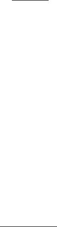
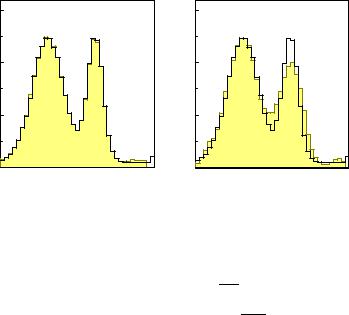
A simple example for the first iteration is sketched in Fig. 9.5. The start distribution in 9.5a for the true histogram has been chosen as uniform. It consists of three bins. Application of the transfer matrix produces 9.5b, a first prediction for the data. The di erent shadings indicate the origin of the entries in the five observed bins. Now the distribution 9.5b is compared with the observed distribution 9.5c. The agreement is bad, for instance the second observed bin di ers from the prediction by a factor two. All contributions of the prediction to this bin are now multiplied by two. Finally the scaled contributions are summed up according to their origin to a new true distribution 9.5d. If there would be only losses, but no migration of entries, this first iteration would lead to a complete correction.

This procedure corresponds to the following equations: The prediction d(k) of the iteration k is obtained from the true vector θ(k):

234 9 Deconvolution

We may now regularize the transfer matrix by suppressing small eigenvalues λi < λmin in D. This means, the corresponding components of the vector

( ˆ) d Ud i

(Uθ)i =

λi

ˆ= −1(d) .

θU Uθ

Instead of cutting abruptly the eigenvalues which are smaller than λmin, it has been proposed to damp their contributions continuously. An advantage of such a procedure is not evident, however.

The choice of the regularization parameter λmin follows the same scheme as for the other methods. The solutions with and without regularization are convoluted and compared with the observed histogram and in both cases χ2 is calculated. The value of χ2 of the regularized solution should exceed the not regularized one not more than allowed statistically.

Often the same bin width is chosen for the true and the observed histogram. It is, however, often appropriate to add at least some marginal bins in the observed histogram which is broader due to the finite resolution. The transfer matrix then becomes rectangular. We have to recast (9.3) somewhat to obtain a quadratic matrix TT T which can be inverted:

TT d = TT Tθ ,

After this transformation the treatment is as above.

9.3 Binning-free Methods

We now present binning-free methods where the observations need not be combined into bins. The deconvolution produces again a sample. The advantage of this approach is that arbitrary histograms under various selection criteria can be constructed afterwards. It is especially suited for low statistics distributions in high dimensional spaces where histograming methods fail.

9.3.1 Iterative Deconvolution

We can realize the iterative weighting method described in Sect. 9.2.2 also in a similar way without binning [52].

We start with a Monte Carlo sample of events, each event being defined by the true coordinate x and the observation x′. During the iteration process we modify at each step a weight which we associate to the events such that the densities in the observation space of simulated and real events approach each other. Initially all weights are equal to one. At the end of the procedure we have a sample of weighted events which corresponds to the deconvoluted distribution.

To this end, we estimate a local density d′(x′i) in the vicinity of any point x′i in the observation space. (For simplicity, we restrict ourselves again to a one-dimensional space since the generalization to several dimensions is trivial.) The following density estimation methods (see Chap. 12) lend themselves:

1.The density is taken as the number of observations within a certain fixed region

around x′i, divided by the length of the region. The length should correspond roughly to the resolution, if the region contains a su cient number of entries.

2.The density is chosen proportional to the inverse length of that interval which contains the K nearest neighbors, where K should be not less than about 10 and should be adjusted by the user to the available resolution and statistics.

We denote by t(x) the simulated density in the true space at location x, by t′(x′) the observed simulated density at x′ and the corresponding data density be d′(x′). The density d′(x′) is estimated from the length of the interval containing K events, t′(x′) from the number of simulated events M(x′) in the same interval. The simulated densities are updated in each iteration step k. We associate a preliminary weight

to the Monte Carlo event i. The weighted events in the vicinity of x represent a new density t(1)(x) in the true space. We now associate a true weight wi to the

event which is just the average over the preliminary weights of all K events in the

P

neighborhood of xi, wi = j wj′ /K. With the smoothed weight wi a new observed

simulated density t′(1)is computed. In the k’th iteration the preliminary weight is given by

The weight will remain constant once the densities t′ and d′ agree. As result we obtain a discrete distribution of coordinates xi with appropriate weights wi, which represents the deconvoluted distribution. The degree of regularization depends on the parameters K used for the density estimation.

The method is obviously not restricted to one-dimensional distributions, and is indeed useful in multi-dimensional cases, where histogram bins su er from small numbers of entries. We have to replace xi, x′i by xi, x′i, and the regions for the density estimation are multi-dimensional.

9.3.2 The Satellite Method

The basic idea of this method [53] is the following: We generate a Monte Carlo sample of the same size as the experimental data sample. We let the Monte Carlo events migrate until the convolution of their position is compatible with the observed data.

236 9 Deconvolution

With the help of a test variable φ, which could for example be the negative log likelihood and which we will specify later, we have the possibility to judge quantitatively the compatibility. When the process has converged, i.e. φ has reached its minimum, the Monte Carlo sample represents the deconvoluted distribution.

We proceed as follows:

We denote by {x′1, . . . , x′N } the locations of the points of the experimental sample and by {y1, . . . , yN } thoseX of the Monte Carlo sample. The observed density of the

simulation is f(y′) =

i

test variable φ [x′1, . . . , x′N ; f(y′)] is a function of the sample coordinates xi and the density expected for the simulation. We execute the following steps:

1.The points of the experimental sample {x′1, . . . , x′N } are used as a first approximation to the true locations y1 = x′1, . . . , yN = x′N .

2.We compute the test quantity φ of the system.

3.We select randomly a Monte Carlo event and let it migrate by a random amount

yi into a randomly chosen direction, yi → yi + yi.

4.We recompute φ. If φ has decreased, we keep the move, otherwise we reject it. If φ has reached its minimum, we stop, if not, we return to step 3.

The resolution or smearing function t is normally not a simple analytic function, but only numerically available through a Monte Carlo simulation. Thus we associate to each true Monte Carlo point i a set of K generated observations {y′i1, . . . , y′iK }, which we call satellites and which move together with yi. The test quantity φ is now a function of the N experimental positions and the N × K smeared Monte Carlo positions.

Choices of the test variable φ are presented in Chap. 10. We recommend to use the variable energy.

The migration distances yi should be taken from a distribution with a width somewhat larger than the measurement resolution, while the exact shape of the distribution is not relevant. We therefore recommend to use a uniform distribution, for which the generation of random numbers is faster than for a normal or other distributions. The result of the deconvolution is independent from these choices, but the number of iteration steps can raise appreciably for a bad choice of parameters.

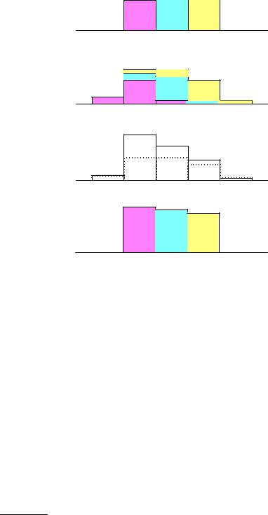
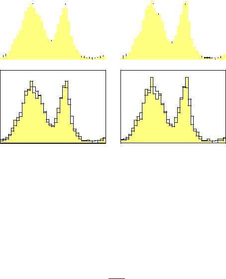
Example 123. Deconvolution of a blurred picture

Figure 9.7 shows a two-dimensional application. The observed picture consisted of lines and points which are convoluted with a two-dimensional normal distribution. In the Monte Carlo simulation for each true point K = 25 satellites have been generated. The energy φ is minimized. The resolution of the lines in the deconvoluted figure on the right hand side is restricted by the low experimental statistics. For the eyes the restriction is predominantly due to the low Monte Carlo factor K. Each eye has N = 60 points. The maximal resolution for a point measured N times is obtained for measurement error σf as