vstatmp_engl
.pdf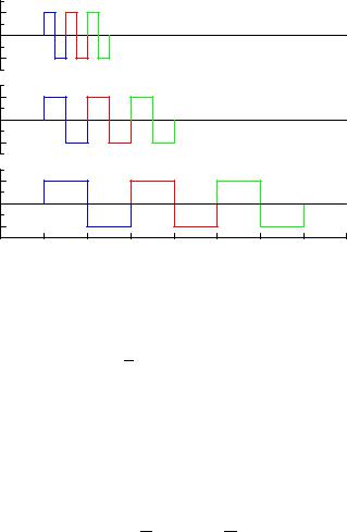

11.2 Smoothing of Measurements and Approximation by Analytic Functions |
301 |
y
x
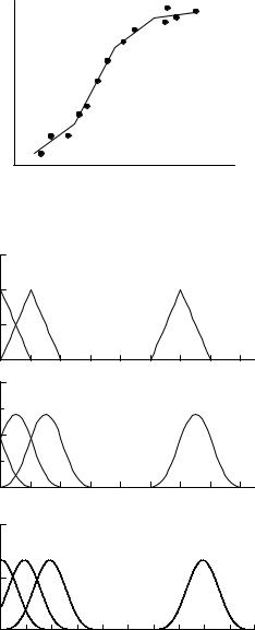
Fig. 11.3. Linear spline approximation.
1.5 |
|
|
|
linear B-splines |
|
y 1.0 |
|
|
0.5 |
|
|
0.0 |
|
|
1.0 |
x |
|
quadratic B-splines |
||
y |
||
|
||
0.5 |
|
|
0.0 |
|
|
|
x |
|
1.0 |
|
cubic B-splines
y0.5
0.0
x
Fig. 11.4. Linear, quadratic and cubic B-splines.
≥ n+1. Since a curve with continuous second derivatives looks smooth to the human eye, splines of degree higher than cubic are rarely used.
Spline approximations are widely used in technical disciplines. They have also been successfully applied to the deconvolution problem [8] (Chap. 9). Instead of adapting a histogram to the true distribution, the amplitudes of spline functions can be fitted. This has the advantage that we obtain a continuous function which incorporates the desired degree of regularization.
For the numerical computations the so called B-splines (basis splines) are especially useful. Linear, quadratic and cubic B-splines are shown in Fig. 11.4. The
302 11 Statistical Learning
superposition of B-splines fulfils the continuity conditions at the knots. The superposition of the triangular linear B-splines produces a polygon, that of quadratic and cubic B-splines a curve with continuous slope and curvature, respectively.
A B-spline of given degree is determined by the step width b and the position x0 of its center. Their explicit mathematical expressions are given in Appendix 13.12.
The function is approximated by
XK
ˆ (11.12) f(x) = akBk(x) .
k=0
The amplitudes ak can be obtained from a least squares fit. For values of the response function yi and errors δyi at the input points xi, i = 1, . . . , N, we minimize
|
|
|
|
|
K |
|
2 |
|
|
|
N |
y |
i − |
akBk(xi) |
i |
|
|
||
|
|
|
|
||||||
|
Xi |
|
k=0 |
|
|
|
|||
χ2 = |
|
h |
|
|
. |
(11.13) |
|||
|
|
|
P |
|
2 |
|
|||
|
=1 |
|
|
(δyi) |
|
|
|
||
|
|
|
|
|
|
|
|
|
|
Of course, the number N of input values has to be at least equal to the number K of splines. Otherwise the number of degrees of freedom would become negative and the approximation under-determined.
Spline Approximation in Higher Dimensions
In principle, the spline approximation can be generalized to higher dimensions. However, there the di culty is that a grid of intervals (knots) destroys the rotation symmetry. It is again advantageous to work with B-splines. Their definition becomes more complicated: In two dimensions we have instead of triangular functions pyramids and for quadratic splines also mixed terms x1x2 have to be taken into account. In higher dimensions the number of mixed terms explodes, another example of the curse of dimensionality.
11.2.5 Approximation by a Combination of Simple Functions
There is no general recipe for function approximation. An experienced scientist would try, first of all, to find functions which describe the asymptotic behavior and the rough distribution of the data, and then add further functions to describe the details. This approach is more tedious than using programs from libraries but will usually produce results superior to those of the general methods described above.
Besides polynomials, a0 + a1x + a2x2 + · · ·, rational functions can be used, i.e. quotients of two polynomials (Padé approximation), the exponential function eαx,
the logarithm b log x, the Gaussian e−ax2 , and combinations like xae−bx. In many cases a simple polynomial will do. The results usually improve when the original data are transformed by translation and dilatation x → a(x + b) to a normalized form.
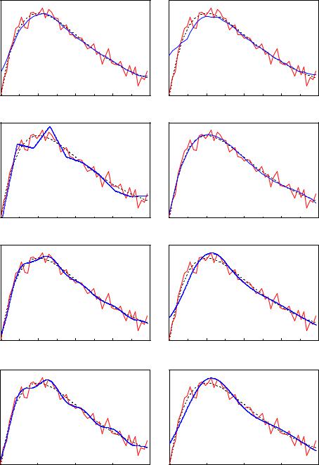
11.2.6 Example
In order to compare di erent methods, we have generated at equidistant values xi of the variable x, function values yi according to the function xe−xwith superimposed
11.3 Linear Factor Analysis and Principal Components |
303 |
Gaussian fluctuations. The measurements generated in this way are smoothed, respectively fitted by di erent functions. The results are shown in Fig. 10.9. All eight panels show the original function and the measured points connected by a polygon.
In the upper two panels smoothing has been performed by weighting. Typical for both methods are that structures are washed-out and strong deviations at the borders. The Gaussian weighting in the left hand panel performs better than the method of nearest neighbors on the right hand side which also shows spurious short range fluctuations which are typical for this method.
As expected, also the linear spline approximation is not satisfactory but the edges are reproduced better than with the weighting methods. Both quadratic and cubic splines with 10 free parameters describe the measurement points adequately, but the cubic splines show some unwanted oscillations. The structure of the spline intervals is clearly seen. Reducing the number of free parameters to 5 suppresses the spurious fluctuations but then the spline functions cannot follow any more the steep rise at small x. There is only a marginal di erence between the quadratic and the cubic spline approximations.
The approximation by a simple polynomial of fourth order, i.e. with 5 free parameters, works excellently. By the way, it di ers substantially from the Taylor expansion of the true function. The polynomial can adapt itself much better to regions of different curvature than the splines with their fixed step width.
To summarize: The physicist will usually prefer to construct a clever parametrization with simple analytic functions to describe his data and avoid the more general standard methods available in program libraries. Those are useful to get a fast overview and for the parametrization of a large amount of data.
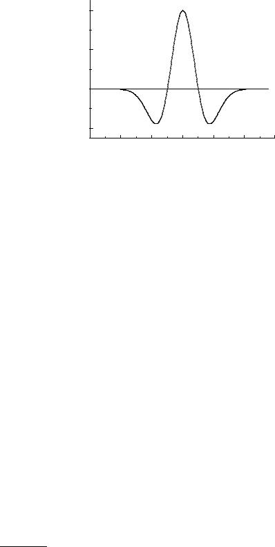
As we have already mentioned, the approximation of measurements by the standard set of orthogonal functions works quite well for very smooth functions where sharp peaks and valleys are absent. Peaks and bumps are better described with wavelets than with the conventional orthogonal functions. Smoothing results of measurements with the primitive kernel methods which we have discussed are usually unsatisfactory. A better performance is obtained with kernels with variable width and corrections for a possible boundary bias. The reader is referred to the literature [86]. Spline approximations are useful when the user has no idea about the shape of the function and when the measurements are able to constrain the function su ciently to suppress fake oscillations.
11.3 Linear Factor Analysis and Principal Components
Factor analysis and principal component analysis (PCA) both reduce a multidimensional variate space to lower dimensions. In the literature there is no clear distinction between the two techniques.
Often several features of an object are correlated or redundant, and we want to express them by a few uncorrelated components with the hope to gain deeper insight into latent relations. One would like to reduce the number of features to as low a number of components, called factors, as possible.
Let us imagine that for 20 cuboids we have determined 6 geometrical and physical quantities: volume, surface, basis area, sum of edge lengths, mass, and principal moments of inertia. We submit these data which may be represented by a 6-dimensional
11.3 Linear Factor Analysis and Principal Components |
305 |
vector to a colleague without further information. He will look for similarities and correlations, and he might guess that these data can be derived for each cuboid from only 4 parameters, namely length, width, height, and density. The search for these basis parameters, the components or factors is called factor analysis [67, 68].
A general solution for this problem cannot be given, without an ansatz for the functional relationship between the feature matrix, in our example build from the 20 six-dimensional data vectors and its errors. Our example indicates though, in which direction we might search for a solution of this problem. Each body is represented by a point in a six-dimensional feature space. The points are, however, restricted to a four-dimensional subspace, the component space. The problem is to find this subspace. This is relatively simple if it is linear.
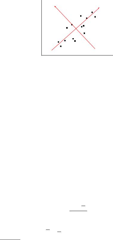
In general, and in our example, the subspace is not linear, but a linear approximation might be justified if the cuboids are very similar such that the components depend approximately linearly on the deviations of the input vectors from a center of gravity. Certainly in the general situation it is reasonable to look first for a linear relationship between features and parameters. Then the subspace is a linear vector space and easy to identify. In the special situation where only one component exists, all points lie approximately on a straight line, deviations being due to measurement errors and non-linearity. To identify the multi-dimensional plane, we have to investigate the correlation matrix. Its transformation into diagonal form delivers the principal components – linear combinations of the feature vectors in the direction of the principal axes. The principal components are the eigenvectors of the correlation matrix ordered according to decreasing eigenvalues. When we ignore the principal components with small eigenvalues, the remaining components form the planar subspace.
Factor analysis or PCA has been developed in psychology, but it is widely used also in other descriptive fields, and there are numerous applications in chemistry and biology. Its moderate computing requirements which are at the expense of the restriction to linear relations, are certainly one of the historical reasons for its popularity. We sketch it below, because it is still in use, and because it helps to get a quick idea of hidden structures in multi-dimensional data. When no dominant components are found, it may help to disprove expected relations between di erent observations.
A typical application is the search for factors explaining similar properties between di erent objects: Di erent chemical compounds may act similarly, e.g. decrease the surface tension of water. The compounds may di er in various features, as molecular size and weight, electrical dipole moment, and others. We want to know which parameter or combination of parameters is relevant for the interesting property. Another application is the search for decisive factors for a similar curing e ect of di erent drugs. The knowledge of the principal factors helps to find new drugs with the same positive e ect.
In physics factor analysis does not play a central role, mainly because its results are often di cult to interpret and, as we will see below, not unambiguous. It is not easy, therefore, to find examples from our discipline. Here we illustrate the method with an artificially constructed example taken from astronomy.
Example 140. Principal component analysis
Galaxies show the well known red-shift of the spectrum which is due to their escape velocity. Besides the measurement value or feature red-shift x1 we know the brightness x2 of the galaxies. To be independent of scales and