vstatmp_engl

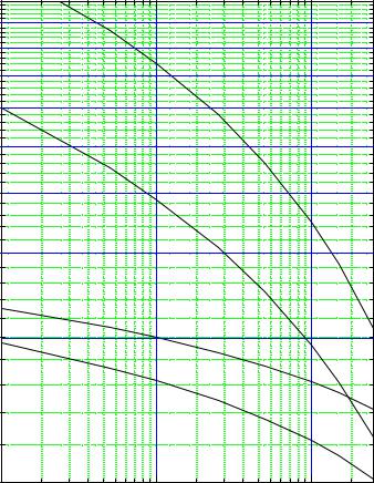
Fig. 13.3. Two hypotheses compared to an observation. The likelihood ratio supports hypothesis 1 while the distance in units of st.dev. supports hypothesis 2.

To keep the discussion simple, we do not exclude negative times t. The earthquake then takes place at time t = 10 h. In Fig. 13.3 are shown both hypothetical distributions in logarithmic form together with the actually observed time. The first prediction H1 di ers by more than one standard deviation from the observation, prediction H2 by less than one standard deviation. Is then H2 the more probable theory? Well, we cannot attribute probabilities to the theories but the likelihood ratio R which here has the value R = 26, strongly supports hypothesis H1. We could, however, also consider both hypotheses as special cases of a third general theory with the parametrization

and now try to infer the parameter θ and its error interval. The observation produces the likelihood function shown in the lower part of Fig. 13.3. The usual likelihood ratio interval contains the parameter θ1 and excludes θ2 while the frequentist standard confidence interval [7.66, ∞] would lead to the reverse conclusion which contradicts the likelihood ratio result and also our intuitive conclusions.

The presented examples indicate that depending on the kind of problem, di erent statistical methods are to be applied.

13.7 P-Values for EDF-Statistics 359

like in many other situations, a uniform prior would be acceptable to most scientists and then the Bayesian interval would coincide with a likelihood ratio interval.

13.6.4 The Likelihood Ratio Approach

To avoid the introduction of prior probabilities, physicists are usually satisfied with the information contained in the likelihood function. In most cases the MLE and the likelihood ratio error interval are su cient to summarize the result. Contrary to the frequentist confidence interval this concept is compatible with the maximum likelihood point estimation as well as with the likelihood ratio comparison of discrete hypotheses and allows to combine results in a consistent way. Parameter transformation invariance holds. However, there is no coverage guarantee and an interpretation in terms of probability is possible only for small error intervals, where prior densities can be assumed to be constant within the accuracy of the measurement.

13.6.5 Conclusion

The choice of the statistical method has to be adapted to the concrete application. The frequentist reasoning is relevant in rare situations like event selection, where coverage could be of some importance or when secondary statistics is performed with estimated parameters. In some situations Bayesian tools are required to proceed to sensible results. In all other cases the presentation of the likelihood function, or, as a summary of it, the MLE and a likelihood ratio interval are the best choice to document the inference result.

13.7 P-Values for EDF-Statistics

The formulas reviewed here are taken from the book of D’Agostino and Stephens [81] and generalized to include the case of the two-sample comparison.

Calculation of the Test Statistics

The calculation of the supremum statistics D and of V = D+ + D− is simple enough, so we will skip a further discussion.

The quadratic statistics W 2, U2 and A2 are calculated after a probability integral transformation (PIT). The PIT transforms the expected theoretical distribution of x into a uniform distribution. The new variate z is found from the relation z = F (x), whereby F is the integral distribution function of x.

With the transformed observations zi, ordered according to increasing values, we get for W 2, U2 and A2:

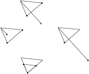
Fig. 13.4. P-values for empirical test statistics.

N

If we know the distribution function not analytically but only from a Monte-Carlo simulation, the z-value for an observation x is approximately z ≈ (number of MonteCarlo observations with xMC < x) /(total number of Monte Carlo observations). (Somewhat more accurate is an interpolation). For the comparison with a simulated distribution is N to be taken as the equivalent number of observations

Here Nexp and NMC are the experimental respectively the simulated sample sizes.

Calculation of p-Values

After normalizing the test variables with appropriate powers of N they follow p.d.f.s which are independent of N. The test statistics’ D , W 2 , A2 modified in this way are defined by the following empirical relations

The relation between these modified statistics and the p-values is given in Fig. 13.7.

13.8 Comparison of two Histograms, Goodness-of-Fit and Parameter Estimation

In the main text we have treated goodness-of-fit and parameter estimation from a comparison of two histograms in the simple situation where the statistical errors of one of the histograms (generated by Monte Carlo simulation) was negligible compared to the uncertainties of the other histogram. Here we take the errors of both histograms into account and also permit that the histogram bins contain weighted entries.

13.8.1 Comparison of two Poisson Numbers with Di erent Normalization

We compare cnn with cmm where the normalization constants cn, cm are known and n, m are Poisson distributed. The null hypothesis H0 is that n is drawn from a distribution with mean λ/cn and m from a distribution with mean λ/cm. We form a χ2 expression

where the denominator δ2 is the expected variance of the parenthesis in the numerator under the null hypothesis.

The log-likelihood of λ is

362 13 Appendix

We compute δ2 under the assumption that n is distributed according to a Poisson

distribution with mean ˆ and respectively, mean ˆ . nˆ = λ/cn mˆ = λ/cm

δ2 = c2nnˆ + c2mmˆ

ˆ

= (cn + cm)λ = cncm(n + m)

and inserting the result into (13.28), we obtain

Notice that the normalization constants are defined up to a common factor, only the relative normalization cn/cm is relevant.

13.8.2 Comparison of Weighted Sums

When we compare experimental data to a Monte Carlo simulation, the simulated events frequently are weighted. We generalize our result to the situation where both numbers n, m consist of a sum of weights. Now the equivalent numbers of events n˜ and m˜ are approximately Poisson distributed. We simply have to replace (13.30) by

n˜ = X , m˜ = X vk2 wk2

and find with c˜nn˜ = cnn, c˜mm˜ = cmm:

13.8.3 χ2 of Histograms

We have to evaluate the expression (13.31) for each bin and sum over all B bins

where the prescription indicated by the index i means that all quantities in the bracket have to be evaluated for bin i. In case the entries are not weighted the tilde is obsolete. The cn, cm usually are overall normalization constants and equal for all bins of the corresponding histogram. If the histograms are normalized with respect to each other, we have cnΣni = cmΣmi and we can set cn = Σmi = M and

cm = Σni = N.

364 13 Appendix

χ2 Parameter Estimation

In principle all weights [wk]i of all bins might depend on θ. We have to minimize (13.32) and recompute all weights for each minimization step. The standard situation is however, that the experimental events are not weighted and that the weights of the Monte Carlo events are equal for all events of the same bin. Then (13.32) simplifies with n˜i = ni, c˜n = cn, c˜m = cmw and m˜ i is just the number of unweighted Monte Carlo events in bin i:

Maximum Likelihood Method

We generalize the binned likelihood fit to the situation with weighted events. We have

We start with a single bin. The probability to observe n˜ (m˜ ) is given by the Poisson

which we have to maximize with respect to the parameters entering into the Monte

Carlo simulation hidden in ˜ .

λ, c˜m, m˜

For the standard case which we have treated in the χ2 fit, we can apply here the same simplifications:

13.9 Extremum Search

If we apply the maximum-likelihood method for parameter estimation, we have to find the maximum of a function in the parameter space. This is, as a rule, not possible without numerical tools. An analogous problem is posed by the method of least squares. Minimum and maximum search are principally not di erent problems, since we can invert the sign of the function. We restrict ourselves to the minimum search.

Before we engage o -the-shelf computer programs, we should obtain some rough idea of their function. The best way in most cases is a graphical presentation. It is not important for the user to know the details of the programs, but some knowledge of their underlying principles is helpful.

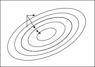
366 13 Appendix

Δλ1

Δλ2 λ2

λ1

Fig. 13.6. Method of steepest descent.

the best point A (13.5c). In each case one of the four configurations is chosen and the iteration continued.

13.9.3 The Parabola Method

Again we begin with starting points in parameter space. In the one-dimensional case we choose 3 points and put a parabola through them. The point with the largest function value is dropped and replaced by the minimum of the parabola and a new parabola is computed. In the general situation of an n-dimensional space, 2n + 1 points are selected which determine a paraboloid. Again the worst point is replaced by the vertex of the paraboloid. The iteration converges for functions which are convex in the search region.

13.9.4 The Method of Steepest Descent

A traveler, walking in a landscape unknown to him, who wants to find a lake, will chose a direction down-hill perpendicular to the curves of equal height (if there are no insurmountable obstacles). The same method is applied when searching for a minimum by the method of steepest descent. We consider this local method in more detail, as in some cases it has to be programmed by the user himself.

We start from a certain point λ0 in the parameter space, calculate the gradientλf(λ) of the function f(λ) which we want to minimize and move by λ downhill.

λ = −α λf(λ) .

The step length depends on the learning constant α which is chosen by the user. This process is iterated until the function remains essentially constant. The method is sketched in Fig. 13.6.

The method of steepest descent has advantages as well as drawbacks: