vstatmp_engl

ln Lumax = −(a + b) + a ln a + b ln b .

Our test statistic is VAB , the logarithm of the likelihood ratio, now summed over all bins:

VAB = ln Lcmax − ln Lumax

= X (ai + bi) ln ai + bi − ai ln ai − bi ln bi + bi ln r . 1 + r

i

Note that VAB (r) = VBA(1/r), as it should.

Now we need a method to determine the expected distribution of the test statistic VAB under the assumption that both samples originate from the same population.

To generate a distribution from a sample, the so-called bootstrap method [64](see Chap. 12.2) has been developed. In our situation a variant of it, a simple permutation method is appropriate.

We combine the two samples to a new sample with M +N elements and form new pairs of samples, the bootstrap samples, with M and N elements by permutation: We draw randomly M elements from the combined sample and associate them to A and the remaining elements to B. Computationally this is easier than to use systematically all individual possibilities. For each generated pair i we determine the statistic Vi. This procedure is repeated many times and the values Vi form the reference distribution. Our experimental p-value is equal to the fraction of generated Vi which are larger than VAB:

p = Number of permutations with Vi > VAB .

10.4.4 The Kolmogorov–Smirnov Test

Also the Kolmogorov–Smirnov test can easily be adapted to a comparison of two

samples. We construct the test statistic in an analogous way as above. The test p

statistic is D = D Neff , where D is the maximum di erence between the two empirical distribution functions SA, SB, and Neff is the e ective or equivalent number of events, which is computed from the relation:

1 = 1 + 1 . Neff N M

In a similar way other EDF multi-dimensional tests which we have discussed above can be adjusted.

10.4.5 The Energy Test

For a binning-free comparison of two samples A and B with M and N observations we can again use the energy test [63] which in the multi-dimensional case has only few competitors.

We compute the energy φAB in the same way as above, replacing the Monte Carlo sample by one of the experimental samples. The expected distribution of the test statistic φAB is computed in the same way as for the likelihood ratio test from

280 10 Hypothesis Tests

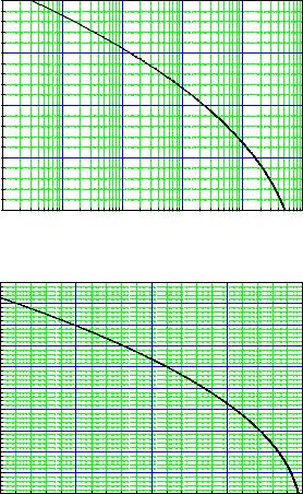
Fig. 10.16. Transformation of p-values to one-sided number of standard deviations.

with some uncertainties in the parameters and assumptions which are di cult to implement in the test procedure. We then have to be especially conservative. It is better to underestimate the significance of a signal than to present evidence for a new phenomenon based on a doubtful number.

To illustrate this problem we return to our standard example where we search for a line in a one-dimensional spectrum. Usually, the background under an observed bump is estimated from the number of events outside but near the bump in the so-called side bands. If the side bands are chosen too close to the signal they are a ected by the tails of the signal, if they are chosen too far away, the extrapolation into the signal region is sensitive to the assumed shape of the background distribution which often is approximated by a linear or quadratic function. This makes it di cult to estimate the size and the uncertainty of the expected background with su cient accuracy to establish the p-value for a large (>4 st. dev.) signal. As numerical example let

us consider an expectation of 1000 background events which is estimated by the experimenter too low by 2%, i.e. equal to 980. Then a 4.3 st. dev. excess would be claimed by him as a 5 st. dev. e ect and he would find too low a p-value by a factor of 28. We also have to be careful with numerical approximations, for instance when we approximate a Poisson distribution by a Gaussian.

Usually, the likelihood ratio, i.e. the ratio of the likelihood which maximizes Hs and the maximum likelihood for H0 is the most powerful test statistic. In some situations a relevant parameter which characterizes the signal strength is more informative.

10.5.2 The Likelihood Ratio Test

Definition

An obvious candidate for the test statistic is the likelihood ratio (LR) which we have introduced and used in Sect. 10.3 to test goodness-of-fit of histograms, and in Sect. 10.4 as a two-sample test. We repeat here its general definition:

λ= sup [L0(θ0|x)] , sup [Ls(θs|x)]

ln λ = ln sup [L0(θ0|x)] − ln sup [Ls(θs|x)]

where L0, Ls are the likelihoods under the null hypothesis and the signal hypothesis, respectively. The supremum is to be evaluated relative to the parameters, i.e. the likelihoods are to be taken at the MLEs of the parameters. The vector x represents the sample of the N observations x1, . . . , xN of a one-dimensional geometric space. The extension to a multi-dimensional space is trivial but complicates the writing of the formulas. The parameter space of H0 is assumed to be a subset of that of Hs. Therefore λ will be smaller or equal to one.

For example, we may want to find out whether a background distribution is described significantly better by a cubic than by a linear distribution:

We would fit separately the parameters of the two functions to the observed data and then take the ratio of the corresponding maximized likelihoods.

Frequently the data sample is so large that we better analyze it in form of a histogram. Then the distribution of the number of events yi in bin i, i = 1, . . . , B can be approximated by normal distributions around the parameter dependent predictions ti(θ). As we have seen in Chap. 6, Sect. 6.5.6 we then get the log-likelihood

plus signal:

The p-value derived from the LR statistic does not take into account that a simple hypothesis is a priori more attractive than a composite one which contains free parameters. Another point of criticism is that the LR is evaluated only at the parameters that maximize the likelihood while the parameters su er from uncertainties. Thus conclusions should not be based on the p-value only.

A Bayesian approach applies so-called Bayes factors to correct for the mentioned e ects but is not very popular because it has other caveats. Its essentials are presented in the Appendix 13.14

Distribution of the Test Statistic

The distribution of λ under H0 in the general case is not known analytically; however, if the approximation (10.27) is justified, the distribution of −2 ln λ under certain additional regularity conditions and the conditions mentioned at the end of Sect. 10.3.3 will be described by a χ2 distribution. In the example corresponding to relations (10.25) this would be a χ2 distribution of 2 degrees of freedom since fs compared to f0 has 2 additional free parameters. Knowing the distribution of the test statistic reduces the computational e ort required for the numerical evaluation of p-values considerably.

Let us look at a specific problem: We want to check whether an observed bump above a continuous background can be described by a fluctuation or whether it corresponds to a resonance. The two hypotheses may be described by the distributions

and we can again use ln λ or Δχ2 as test statistic. Since we have to define the test before looking at the data, µ and σ will be free parameters in the fit of fs to the data. Unfortunately, now Δχ2 no longer follows a χ2 distribution of 3 degrees of freedom and has a significantly larger expectation value than expected from the χ2 distribution. The reason for this dilemma is that for α3 = 0 which corresponds to H0 the other parameters µ and σ are undefined and thus part of the χ2 fluctuation in the fit to fs is unrelated to the di erence between fs and f0.

More generally, only if the following conditions are satisfied, Δχ2 follows in the large number limit a χ2 distribution with the number of degrees of freedom given by the di erence of the number of free parameters of the null and the alternative hypotheses:

1.The distribution f0 of H0 has to be a special realization of the distribution fs of

Hs.

2.The fitted parameters have to be inside the region, i.e. o the boundary, allowed by the hypotheses. For example, the MLE of the location of a Gaussian should not be outside the range covered by the data.

3.All parameters of Hs have to be defined under H0.

284 10 Hypothesis Tests

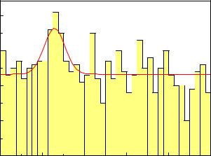
Fig. 10.18. Histogram of event sample used for the likelihood ratio test. The curve is an unbinned likelihood fit to the data.

claim large e ects. Figure 10.18 displays the result of an experiment where a likelihood fit finds a resonance at the energy 0.257. It contains a fraction of 0.0653 of the events. The logarithm of the likelihood ratio is 9.277. The corresponding p-value for H0 is pLR = 1.8 · 10−4. Hence it is likely that the observed bump is a resonance. In fact it had been generated as a 7 % contribution of a Gaussian distribution N(x|0.25, 0.05) to a uniform distribution.

We have to remember though that the p-value is not the probability that H0 is true, it is the probability that H0 simulates the resonance of the type seen in the data. In a Bayesian treatment, see Appendix 13.14, we find betting odds in favor of H0 of about 2% which is much less impressive. The two numbers refer to di erent issues but nonetheless we have to face the fact that the two di erent statistical approaches lead to di erent conclusions about how evident the existence of a bump really is.

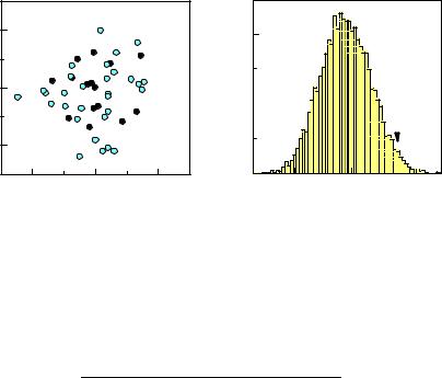
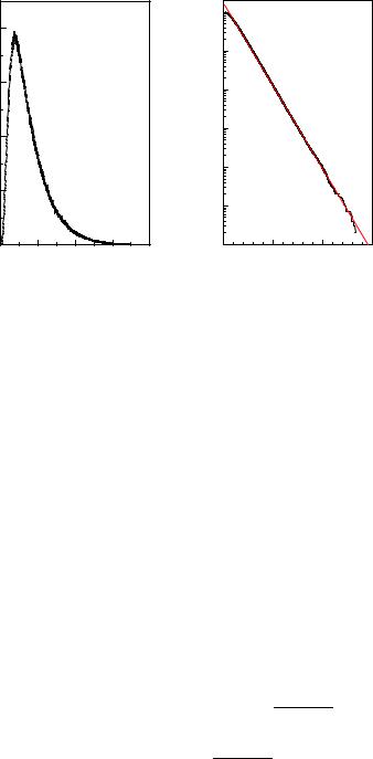
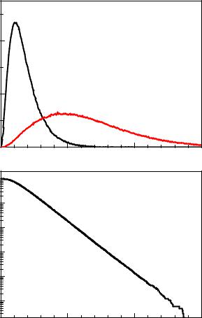
In experiments with a large number of events, the computation of the p-value distribution based on the unbinned likelihood ratio becomes excessively slow and we have to turn to histograms and to compute the likelihood ratio of H0 and Hs from the histogram. Figure 10.19 displays some results from the simulation of 106 experiments of the same type as above but with 10000 events distributed over 100 bins.

In the figure also the distribution of the signal fraction under H0 and for experiments with 1.5% resonance added is shown. The large spread of the signal distributions reflects the fact that identical experiments by chance may observe a very significant signal or just a slight indication of a resonance.

286 10 Hypothesis Tests

When we denote the decay contribution into channel k by εk, the p.d.f. of the decay distribution by fk(xk|θk) and the corresponding background distributions by f0k(xk|θ0k), the distribution under H0 is

YK

f0(x1, . . . , xK |θ01, . . . , θ0K ) = f0k(xk|θ0k)

k=1

and the alternative signal distribution is

fs(x1, . . . , xK |θ01, . . . , θ0K ; θ1, . . . , θK ; ε1, . . . , εK ) =

YK

[ (1 − εk)f0k(xk|θ0k) + εkfk(xk|θk)] .

k=1

Remark, that the MLEs of the parameters θ0k depend on the hypothesis. They are di erent for the null and the signal hypotheses and, for this reason, have been marked by an apostrophe in the latter.

10.5.3 Tests Based on the Signal Strength

Instead of using the LR statistic it is often preferable to use a parameter of Hs as test statistic. In the simple example of (10.25) the test statistic t = α3 would be a sensible choice. When we want to estimate the significance of a line in a background distribution, instead of the likelihood ratio the number of events which we associate to the line (or the parameter α3 in our example (10.28)) is a reasonable test statistic. Compared to the LR statistic it has the advantage to represent a physical parameter but usually the corresponding test is less powerful.

Example 134. Example 133 continued

Using the fitted fraction of resonance events as test statistic, the p-value for H0 is pf = 2.2 · 10−4, slightly less stringent than that obtained from the LR. Often physicists compare the number of observed events directly to the prediction from H0. In our example we have 243 events within two standard deviations around the fitted energy of the resonance compared to the expectation of 200 from a uniform distribution. The probability to observe ≥ 243 for a Poisson distribution with mean 200 is pp = 7.3 · 10−4. This number cannot be compared directly with pLR and pf because the latter two values include the look-else-where e ect, i.e. that the simulated resonance may be located at an arbitrary energy. A lower number for pp is obtained if the background is estimated from the side bands, but then the computation becomes more involved because the error on the expectation has to be included. Primitive methods are only useful for a first crude estimate.

We learn from this example that the LR statistic provides the most powerful test among the considered alternatives. It does not only take into account the excess of events of a signal but also its expected shape. For this reason pLR is smaller than pf .