vstatmp_engl

A sample of space points (xi, yi), i = 1, . . . , N follow a normal distribution

with θ the parameter which we are interested in. The normalized x distribution depends only on θ. Whatever value ν takes, the shape of this distribution remains always the same. Therefore we can estimate θ independently of ν. The likelihood function is proportional to a normal distribution of θ,

6.9.3 Parameter Transformation, Restructuring

Sometimes we manage by means of a parameter transformation ν′ = ν′(θ, ν) to bring the p.d.f. into the desired form (6.33) where the p.d.f. factorizes into two parts which depend separately on the parameters θ and ν′. We have already sketched an example in Sect. 4.3.6: When we are interested in the slope θ and not in the intersection ν with the y-axis of a straight line y = θx + ν which should pass through measured points, then we are able to eliminate the correlation between the two parameters. To this end we express the equation of the straight line by the slope and the ordinate at the center of gravity, see Example 114 in Chap. 7.

A simple transformation ν′ = c1ν + c2θ also helps to disentangle correlated pa-

With suitable chosen constants c1, c2 it produces a likelihood function that factorizes

in the new parameter pair ′. In the notation where the quantities ˆ maximize

θ, ν θ, νˆ the likelihood function, the transformation produces the result

− a2 − ˆ 2

Lθ(θ) exp 2 (θ θ) .

We set the proof of this assertion aside.

It turns out that this procedure yields the same result as simply integrating out the nuisance parameter and as the profile likelihood method which we will discuss below. This result is interesting in the following respect: In many situations the likelihood function is nearly of Gaussian shape. As is shown in Appendix 13.3, the likelihood function approaches a Gaussian with increasing number of observations. Therefore, integrating out the nuisance parameter, or better to apply the profile likelihood method, is a sensible approach in many practical situations. Thus nuisance parameters are a problem only if the sample size is small.

The following example is frequently discussed in the literature [16].

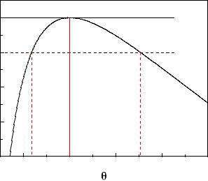
Fig. 6.16. Log-likelihood function of an absorption factor.

Example 100. Elimination of a nuisance parameter by restructuring: absorption measurement

The absorption factor θ for radioactive radiation by a plate is determined from the numbers of events r1 and r2, which are observed with and without the absorber within the same time intervals. The numbers r1, r2 follow Poisson distributions with mean values ρ1 and ρ2:

The interesting parameter is the expected absorption θ = ρ2/ρ1. In first approximation we can use the estimates r1, r2 of the two independent parameters ρ1 and ρ2 and their errors to calculate in the usual way through error propagation θ and its uncertainty:

For large numbers r1, r2 this method is justified but the correct way is to transform the parameters ρ1, ρ2 of the combined distribution

into the independent parameters θ = ρ2/ρ1 and ν = ρ1 + ρ2. The transformation yields:

L(θ, ν|r1, r2) = Lν (ν|r1, r2)Lθ(θ|r1, r2) .

Thus the log-likelihood function of θ is

ln Lθ(θ|r1, r2) = −r1 ln(1 + 1/θ) − r2 ln(1 + θ) .

It is presented in Fig. 6.16 for the specific values r1 = 10, r2 = 20. The

maximum is located at ˆ , as obtained with the simple estimation

θ = r2/r1

above. However the errors are asymmetric.

Instead of a parameter transformation it is sometimes possible to eliminate the nuisance parameter if we can find a statistic y which is independent of the nuisance parameter ν, i.e. ancillary with respect to ν, but dependent on the parameter θ. Then we can use the p.d.f. of y, f(y|θ), which per definition is independent of ν, to estimate θ. Of course, we may loose information because y is not necessarily a su cient statistic relative to θ. The following example illustrates this method. In this case there is no loss of information.

Example 101. Eliminating a nuisance parameter by restructuring: Slope of a straight line with the y-axis intercept as nuisance parameter

We come back to one of our standard examples which can, as we have indicated, be solved by a parameter transformation. Now we solve it in a simpler way. Points (xi, yi) are distributed along a straight line. The x coordinates are exactly known, the y coordinates are the variates. The p.d.f. f(y1, ...yn|θ, ν) contains the slope parameter θ and the uninteresting intercept ν of the line with the y axis. It is easy to recognize that the statistic

{y˜1 = y1 − yn, y˜2 = y2 − yn, . . . , y˜n−1 = yn−1 − yn} is independent of ν. In this specific case the new statistic is also su cient relative to the slope θ

which clearly depends only on the di erences of the ordinates. We leave the details of the solution to the reader.

Further examples for the elimination of a nuisance parameter by restructuring have been given already in Sect. 6.5.2, Examples 79 and 80.

6.9.4 Profile Likelihood

We now turn to approximate solutions.

Some scientists propose to replace the nuisance parameter by its estimate. This corresponds to a delta function for the prior of the nuisance parameter and is for that reason quite exotic and dangerous. It leads to an illegitimate reduction of the error limits whenever the nuisance parameter and the interesting parameter are correlated. Remark, that a correlation always exists unless a factorization is possible. In the extreme case of full correlation the error would shrink to zero.

A much more sensible approach to eliminate the nuisance parameter uses the socalled profile likelihood [33]. To explain it, we give an example with a single nuisance parameter.

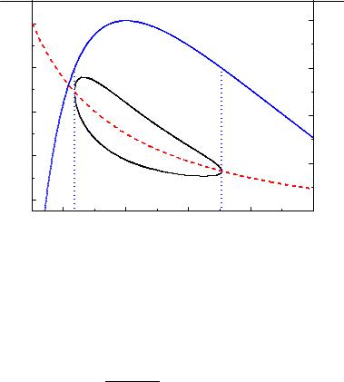
Fig. 6.17. Profile likelihood (solid curve, right hand scale) and ln L(θ, ν) = 1/2 contour (left hand scale). The dashed curve is νˆ(θ).

The likelihood function is maximized with respect to the nuisance parameter ν as a function of the wanted parameter θ. The function νˆ(θ) which maximizes L then

satisfies the relation

∂L(θ, ν|x) |νˆ = 0 → νˆ(θ) . ∂ν

It is inserted into the likelihood function and provides the profile likelihood Lp,

Lp = L (θ, νˆ(θ)|x) ,

which depends solely on θ.

This method has the great advantage that only the likelihood function enters and no assumptions about priors have to be made. It also takes correlations into account. Graphically we can visualize the error interval of the profile likelihood ln Lp(θ, ν) = 1/2 by drawing the tangents of the curve ln L = 1/2 parallel to the ν axis. These tangents include the error interval.

An example of a profile likelihood is depicted in Fig. 6.17. We have used the absorption example from above to compute the curves. The nuisance parameter is ρ1. The result is the same as with the exact factorization.

In the literature we find methods which orthogonalize the parameters at the maximum of the likelihood function [35] which means to diagonalize a more dimensional Gaussian. The result is similar to that of the profile likelihood approach.

In the limit of a large number of observations where the likelihood function approaches the shape of a normal distribution, the profile likelihood method is identical to restructuring and factorizing the likelihood.

6.9.5 Integrating out the Nuisance Parameter

If the methods fail which we have discussed so far, we are left with only two possibilities: Either we give up the elimination of the nuisance parameter or we integrate it out. The simple integration

Z ∞

Lθ(θ|x) = L(θ, ν|x)dν

−∞

implicitly contains the assumption of a uniform prior of ν and therefore depends to some extend on the validity of this condition. However, in most cases it is a reasonable approximation. The e ect of varying the prior is usually negligible, except when the likelihood function is very asymmetric. Also a linear term in the prior does usually not matter. It is interesting to notice that in most cases integrating out the nuisance parameter leads to the same result as restructuring the problem.

6.9.6 Explicit Declaration of the Parameter Dependence

It is not always possible to eliminate the nuisance parameter in such a way that the influence of the method on the result can be neglected. When the likelihood function has a complex structure, we are obliged to document the full likelihood function. In many cases it is possible to indicate the dependence of the estimate θ and its error limits θ1, θ2 on the nuisance parameter ν explicitly by a simple linear function

θ1,2 = θ1,2 + c(ν − νˆ) .

Usually the error limits will show the same dependence as the MLE which means that the width of the interval is independent of ν.

However, publishing a dependence of the parameter of interest on the nuisance parameter is useful only if ν corresponds to a physical constant and not to an internal parameter of an experiment like e ciency or background.

6.9.7 Advice

If it is impossible to eliminate the nuisance parameter explicitly and if the shape of the likelihood function does not di er dramatically from that of a Gaussian, the profile likelihood approach should be used for the parameter and interval estimation. In case the deviation from a Gaussian is considerable, we will try to avoid problems by an explicit declaration of the dependence of the likelihood estimate and limits on the nuisance parameter. If also this fails, we abstain from the elimination of the nuisance parameter and publish the full likelihood function.

7

Parameter Inference II

7.1 Likelihood and Information

7.1.1 Su ciency

In a previous example, we have seen that the likelihood function for a sample of exponentially distributed decay times is a function only of the sample mean. In fact, in many cases, the i.i.d. individual elements of a sample {x1, . . . , xN } can be combined to fewer quantities, ideally to a single one without a ecting the estimation of the interesting parameters. The set of these quantities which are functions of the observations is called a su cient statistic. The sample itself is of course a su cient, while uninteresting statistic.

According to R. A. Fisher, a statistic is su cient for one or several parameters, if by addition of arbitrary other statistics of the same data sample, the parameter estimation cannot be improved. More precise is the following definition [1]: A statistic

t(x1, . . . , xN ) ≡ {t1(x1, . . . , xN ), . . . , tM (x1, . . . , xN )} is su cient for a parameter set

θ, if the distribution of a sample {x1, . . . , xN }, given t, does not depend on θ:

The distribution g(t|θ) then contains all the information which is relevant for the parameter estimation. This means that for the estimation process we can replace the sample by the su cient statistic. In this way we may reduce the amount of data considerably. In the standard situation where all parameter components are constraint by the data, the dimension of t must be larger or equal to the dimension of the parameter vector θ. Every set of uniquely invertible functions of t is also a su cient statistic.

The relevance of su ciency is expressed in a di erent way in the so-called su - ciency principle:

If two di erent sets of observations have the same values of a su cient statistic, then the inference about the unknown parameter should be the same.

Of special interest is a minimal su cient statistic. It consists of a minimal number of components, ideally only of one element per parameter.

In what follows, we consider the case of a one-dimensional su cient statistic t(x1, . . . , xN ) and a single parameter θ. The likelihood function can according to

186 7 Parameter Inference II

The conditionality principle seems to be trivial. Nevertheless the belief in its validity is not shared by all statisticians because it leads to the likelihood principle with its far reaching consequences which are not always intuitively obvious.

7.1.3 The Likelihood Principle

We now discuss a principle which concerns the foundations of statistical inference and which plays a central role in Bayesian statistics.

The likelihood principle (LP) states the following:

Given a p.d.f. f(x|θ) containing an unknown parameter of interest θ and an observation x, all information relevant for the estimation of the parameter θ is contained in the likelihood function L(θ|x) = f(x|θ).

Furthermore, two likelihood functions which are proportional to each other, contain the same information about θ. The general form of the p.d.f. is considered as irrelevant. The p.d.f. at variate values which have not been observed has no bearing for the parameter inference.

Correspondingly, for discrete hypotheses Hi the full experimental information relevant for discriminating between them is contained in the likelihoods Li.

The following examples are intended to make plausible the LP which we have implicitly used in Chap. 6.

Example 105. Likelihood principle, dice

We have a bag of biased dice of type A and B. Dice A produces the numbers 1 to 6 with probabilities 1/12, 1/6, 1/6, 1/6, 1/6, 3/12. The corresponding probabilities for dice B are 3/12, 1/6, 1/6, 1/6, 1/6, 1/12. The result of an experiment where one of the dice is selected randomly is “3”. We are asked to bet for A or B. We are unable to draw a conclusion from the observed result because both dice produce this number with the same probability, the likelihood ratio is equal to one. The LP tells us – what intuitively is clear

– that for a decision the additional information, i.e. the probabilities of the two dice to yield values di erent from “3”, are irrelevant.

Example 106. Likelihood principle, V − A

We come back to an example which we had discussed already in Sect. 6.3. An experiment investigates τ− → µ−ντ ν¯µ, µ− → e−νµν¯e decays and measures the slope αˆ of the cosine of the electron direction with respect to the muon direction in the muon center-of-mass. The parameter α depends on the τ − µ coupling. Is the τ decay proceeding through V −A or V +A coupling? The LP implies that the probabilities f−(α), f+(α) of the two hypotheses to produce values α di erent from the observed value αˆ do not matter.

When we now allow that the decay proceeds through a mixture r = gV /gA of V and A interaction, the inference of the ratio r is based solely on the observed value αˆ, i.e. on L(r|αˆ).

The LP follows inevitably from the su ciency principle and the conditioning principle. It goes back to Fisher, has been reformulated and derived several times