

vstatmp_engl
.pdf
|
|
|
4.2 Di erent Types of Measurement Uncertainty |
87 |
|||
the factor |
√ |
|
|
√ |
|
|
|
|
5 |
than that of a single measurement, δx |
= δx/ 5. With only 5 |
|
|||
repetitions the precision of the error estimate is rather poor.
√
Our recipe yields δx 1/ N, i.e. the error becomes arbitrarily small if the num-
√
ber of the measurements approaches infinity. The validity of the 1/ N behavior relies on the assumption that the fluctuations are purely statistical and that correlated systematic variations are absent, i.e. the data have to be independent of each other. When we measure repeatedly the period of a pendulum, then the accuracy of the measurements can be deduced from the variations of the results only if the clock is not stopped systematically too early or too late and if the clock is not running too fast or too slow. Our experience tells us that some correlation between the di erent measurements usually cannot be avoided completely and thus there is a lower limit for δx. To obtain a reliable estimate of the uncertainty, we have to take care that the systematic uncertainties are small compared to the statistical error δx.
Error of the Empirical Variance
Sometimes we are interested in the variance of an empirical distribution and in its uncertainty. In the same category falls the problem to estimate the error of the error of a parameter which is determined from a series of measurements. For example, we may need to know the resolution of a meter or the width of a spectral line and the related accuracy. It is also of interest to know how often a calibration measurement has to be performed to estimate the corresponding error with su cient accuracy. In these situations the variance s2 itself is the result of the investigation to which we would like to associate an uncertainty.
The variance of (x − µ)2 for a given distribution is easily calculated using the formulas of Sect. 3.2.3. We omit the details of the calculation and quote the result which is related of the second and fourth central moments.
var[(x − µ)2] = D (x − µ)2 − σ2 2E
= (µ′4 − σ4) .
We now assume that our sample is large and replace the distribution moments µ′n by the empirical central moments m′n,
m′n = N1 X(xi − x)n .
The moment s2 = m′2 is an estimate for σ2. For N events in the sample, we get for the uncertainty δs2 of s2
m′ − m′2
(δs2)2 = 4 2
N
and from error propagation (see next section 4.3) we derive the uncertainty of s itself
δs |
|
1 δs2 |
|
|
|
||||||
|
= |
|
|
|
|
, |
|
|
|
||
s |
2 |
s2 |
|
|
|
||||||
|
|
1 |
|
|
p |
m4′ |
s4 |
||||
|
= |
2√ |
|
|
s2− |
|
. |
||||
|
N |
||||||||||
If the type of distribution is known, we can use relations between moments. Thus, for the normal distribution we have µ′4 = 3σ4 (see Sect. 3.6.5), and it follows

88 4 Measurement errors
√
δs/s = 1/ 2N which also follows from the variance of the χ2 distribution. This relation sometimes is applied to arbitrary distributions. It then often underestimates the uncertainty.
4.2.2 Systematic Errors (G. Bohm)
A stringent requirement on scientific results is the possibility of verification or refutation. In case of experiments, the most direct way, indispensable in case of crucial experiments, is their independent repetition. Experimental results have to be presented in a way which allows this: First of all, any experimental number has to be given together with its statistical error. Only then we can state “agreement within errors” and combine the results to a more accurate one, or, not so seldom as one might wish, we find the result “unconfirmed” and the experimental situation “still unclear”.
A cornerstone in such comparisons is the assumption of statistical independence: Statistical fluctuations in the two experiments “have nothing to do with each other”. Anticipating later developments on error propagation for independent variates, we compare the squared di erence of the two results, |x1 − x2|2 with the variance of x1 − x2, given by
var(x1 − x2) = var(x1) + var(x2) − 2cov(x1, x2)
or in terms of the covariance matrix, see Chap. 3, Sect. 3.5.6
var(x1 − x2) = C11 + C22 − 2C12 .
Using independence of the xi, we have C12 = 0 and the diagonal elements of C are the squared errors δx21,2; so, confirmation means
|x1 − x2|2 ≤ k(C11 + C22) |
(4.4) |
with k of order unity4.
The next step is usually the combination of the two results as a weighted mean. This will be explained in the next section; here we anticipate that the error of the combined result will be smaller than the minimum of δx1 and δx2. So, under the assumption of independence, there is no lower limit to the statistical error of repeatable experiments.
Of course, in reality there is always a limit on statistical accuracy, besides the trivial one that time for repetitions is limited: The assumption of independence is violated in a very specific way by so-called systematic errors which appear in any realistic experiment. Postponing an abstract definition we first give some examples to illustrate the usage of this term in physical applications.
1.Reading error of an analog instrument: The readings performed by an observer will not average to the true value, but show a personal bias. This e ect may be estimated by comparing the results of several observers.
4This is of course a rough statement, to be qualified by probabilistic statements if required.

4.2 Di erent Types of Measurement Uncertainty |
89 |
2.Calibration errors of the measurement apparatus: The art of measuring with analog instruments is merely history, since digital displays replaced them. Corrections, like zero shifts, non-linearities etc. are usually taken care of already in the displayed value, but the applier should know, besides the resolution, also the limit of accuracy of the average result for a large sample.
3.Errors of auxiliary quantities: Besides calibration constants, many other physical quantities will influence the final result, all being subject to measurement errors (particle characteristics, former experimental results...)
4.Errors of auxiliary quantities of theoretical origin: Sometimes it is not possible to reach the required accuracy in theoretical calculations of such quantities. Also then an uncertainty should be given, corresponding to a variance in a Bayesian sense.
5.Uncertainties in the definition of the quantity to be measured: A measurement result usually depends, besides from the quantity one wants to measure, on surrounding conditions like temperature or pressure. The size of a body is welldefined only for certain values of these parameters.
6.Errors of parameters determining the statistical model describing the data: Often the parameter of interest is found by adapting a model which depends on this parameter, to the data. Usually such model depends also on other, uninteresting, parameters, called nuisance parameters in statistics, which often cannot be derived from the data alone, but need external input with unavoidable uncertainties.
The above items are neither non-overlapping nor complete. The following is an attempt to give a more formal characterization of systematic errors, meeting, hopefully, the general usage of this denotation.
Let us consider a measured quantity x with statistical error δx. To describe a realistic situation, the final, corrected result x˜ is a function u of x and other, generally also uncertain, auxiliary parameters a, b, . . .: Then a first measurement of x gives
x˜1 = u(x1, a, b, . . .) .
A repeated measurement, presumably under the same conditions, of x yields x2 and
x˜2 = u(x2, a, b, . . .)
with the same unchanged values5 of a, b, . . .. Taylor-expanding u around the expected values hxi, hai, hbi . . . and writing Δxi = xi − hxi, ux = ∂u/∂x etc., we get (in linear approximation)
x˜i = uxΔxi + uaΔa + ubΔb + · · · .
Assuming, for simplicity, all variates on the right hand side as uncorrelated, we find, after squaring and taking expectation values
var(˜xi) = u2xvar(xi) + u2avar(a) + u2b var(b) + · · · , cov(˜x1, x˜2) = u2avar(a) + u2b var(b) + · · · .
The corrected covariance matrix is no longer diagonal. The results of repetitions are not independent, just because they are subject to the same “systematic” e ects from fluctuations of a, b, . . .:
5Besides x1, x2 also their statistical errors may di er.
90 |
4 Measurement errors |
|
|
|
|
|||
|
C˜ = ux2 |
|
var(x ) |
0 |
|
+ [ua2var(a) + ub2var(b) + · · ·] |
1 1 |
. |
|
0 1 |
var(x2) |
1 1 |
|||||
This covariance matrix describes the uncertainty of a doubled measurement completely. The second matrix (of rank unity) expresses the fact that the two measurements are totally positively correlated with respect to the fluctuations of the auxiliary parameters a, b, . . .. The square root of the term in square brackets is
called systematic error and customarily given separately from the “statistical” er-
p
ror δxstati = var(xi). Even more recommendable is the practice to give the list of the systematic errors taken into account, i.e. the values a ± δa, uaδa, the same for
b, and so on. The main advantage of this separation is that it gives the information on how far the accuracy can be enhanced by repetitions of the experiment. A second argument against mixing up statistical and systematic errors is the fact that in practice the latter are often less well known.
Coming back to the comparison of two independent measurements of x under “apparently the same conditions” (4.4), we see that this criterium remains the same, whether or not the identical systematic errors are taken into account. When combining the results, however, the systematic error stays constant. A nasty consequence from this is that systematic errors not taken into account do not signal their existence by larger fluctuations of the data. It is an important part of experimental work to check carefully for any source of systematic errors, and to document every parameter of potential influence.
4.2.3 Systematic Errors (G. Zech)
Introduction and Definition
Experiments in nuclear and particle physics usually extract the information from a statistical data sample. The precision of the results then is mainly determined by the number N of collected reactions. Besides the corresponding well defined statistical errors, nearly every measurement is subject to further uncertainties, the systematic errors, typically associated with auxiliary parameters related to the measuring apparatus, or with model assumptions. The result is typically presented in the form
x = 2.34 ± 0.06 = 2.34 ± 0.05(stat.) ± 0.03(syst.).
The only reason for the separate quotation of the two uncertainties is that the size of the systematic uncertainties is less well known than that of the purely statistical error. Thus, for example, excluding a prediction by say a 4 standard deviation measurement where the errors are dominantly of systematic type is certainly less convincing than if the result is purely statistical.
To illustrate the di erent quality of purely statistical errors and systematic errors, imagine we read a pico-ampere meter. The needle is quivering and sometimes large amplitudes occur due to pick-up. Observing the movement of the needle for some time, we will be able to estimate the current and to guess the uncertainty. Repeating the measurement many times will not sizably reduce the error. A tape-measure may have expanded or shrunk due to temperature e ects. The corresponding uncertainty can be estimated roughly from the estimated range of temperature variations and the known expansion coe cient of the tape material if it is made out of metal. It may also be guessed from previous experience. Characteristic of most systematic errors is that repeated measurements are generally correlated and thus the accuracy

4.2 Di erent Types of Measurement Uncertainty |
91 |
is not improved by a repetition. However, there are other systematic errors where a repetition of a measurement is impossible, for instants when an auxiliary parameter is taken from a technical data sheet or when the measurement has happened in the past. It may happen that we have to derive a parameter from two or three independent and thus uncorrelated observations following an unknown distribution. For instance, the current of a magnet may have been measured at the beginning and at the end of an experiment. The variation of the current introduces an error for the momentum measurement of charged particles. The estimate of the uncertainty from only two measurement will be rather vague and thus the error is of type systematic.
From these considerations follow the definitions:
Statistical errors are determined by objective statistical procedures. They follow a known distribution like a Poisson rate or are determined empirically from the
distribution of an unbiased, su ciently large sample. They show the typical reduction
√
of the error with 1/ N where N is the sample size.
On the contrary, systematic errors cannot be calculated solely from sampling fluctuations and are at least partially based on assumptions made by the experimenter, are model dependent or follow unknown distributions. Thus, the systematic error and / or its distribution are only vaguely known.
√
Most systematic errors do not share the 1/ N law of the statistical errors, but there are exceptions and many systematic errors can be reduced with increasing statistics of an experiment.
Systematic errors arise in most experiments. They are especially important in high precision measurements like those of the magnetic dipole moment of the muon or of the CP violation constants in the neutral kaon system.
Examples of Systematic Errors
Systematic uncertainties arise typically when instruments are poorly calibrated, or are influenced, in a way not known exactly, by the environment (temperature, pressure. . . ), or if thresholds or base levels are not constant in time. Besides uncertainties regarding the measuring instruments, often the knowledge or the understanding of parts of experimental setup, its acceptance and the sensitivity of detector components is incomplete. These e ects and only partially known background contributions lead to systematic errors. Sometimes the data analysis requires additional experimental input from other experiments or theoretical results have to be used, where especially the latter may have uncertainties of unclear nature.
In some of these examples there is no “N”, i.e. there is no possibility to produce several independent guesses, or a repetition of the measurement would not produce an independent result. It does not make sense to repeat the estimate of theoretical uncertainties arising for instance from neglecting higher order terms in an expansion. Sometimes the reason of the uncertainty lies in the past, the failure of some electronic part or the physicist has forgotten to record the atmospheric pressure which influences some calibration constant. Other uncertainties like those of background subtraction can be reduced with increasing statistics, but nevertheless there remains some systematic uncertainty from an extrapolation. Often the measurement of an interesting parameter is correlated with the value of another uninteresting parameter. We call it a nuisance parameter. The uncertainty of the nuisance parameter can
92 4 Measurement errors
induce a systematic uncertainty on the interesting parameter which in first order
√
decreases like 1/ N with the number of observations.
How to Detect and Avoid Systematic Errors
In order to detect and to estimate systematic errors, experience, common sense, and intuition is needed. A general advice is to try to suppress them as far as possible already by an appropriate design of the experiment and to include the possibility of control measurements, like regular calibration. Since correlation of repeated measurement is characteristic for the presence of systematic errors, observed correlations of results with parameters related to the systematic e ects provide the possibility to estimate and reduce the latter. In the pendulum example discussed above the systematic contribution to the error due to a possible unknown bias in the stopping procedure can be estimated by studying the result as a function of the number of periods and reduced by increasing the measurement time. In particle physics experiments where usually only a fraction of events is accepted by some filtering procedure, it is advisable to record also a fraction of those events that are normally rejected (downscaling) and to try to understand their nature. Some systematic e ects are related to the beam intensity, thus a variation of the beam intensity helps to study them.
How can we detect systematic errors caused for instance by background subtraction or e ciency corrections at the stage of data analysis? A widely used method is the investigation of the results as a function of the selection criteria. A correlation of the interesting parameter with the value of a cut-o parameter in a certain variable is a clear indication for the presence of systematic errors. It is evident though that the systematic errors then have to be much larger than the normal statistical fluctuations in order to be detected. Obviously, we want to discriminate also systematic errors which are of the same order of magnitude as the statistical ones, preferably much smaller. Therefore we have to investigate samples, where the systematic e ects are artificially enhanced. If we suspect rate dependent distortion e ects as those connected with dead times, it is recommended to analyze a control sample with considerably enhanced rate. When we eliminate a background reaction by a selection criterion, we should investigate its importance in the region which has been excluded, where it is supposed to be abundant.
Frequently made mistakes are: 1. From the fact that the data are consistent with the absence of systematic errors, it is supposed that they do not exist. This leads always to underestimation of systematic errors. 2. The changes of the results found by changing the selection criteria are directly converted into systematic errors. This in most cases leads to overestimates, because the variations are partially due to the normal statistical fluctuations.
Treatment of Systematic Errors
Because of the di culty to specify systematic errors accurately, scientists are rather sceptical about results based on measurements which are dominated by systematic errors. In any case, it is indispensable to declare the systematic and the statistical contributions to the measurement error separately.
In many experiments there appears a quite large number – typically a dozen or so – of such systematic uncertainties. When we combine systematic errors (see Sect.

4.2 Di erent Types of Measurement Uncertainty |
93 |
8.2), we can often profit from the central limit theorem (see Sect. 3.6.5) provided that they are all of the same order of magnitude. The distribution of the sum of variables su ering from systematic uncertainties approaches a normal distribution, with variance equal to the sum of variances of the contributing distributions. If the variables enter multiplicative, the logarithms are additive and approach a normal distribution (see Sect. 8.2)
Sometimes systematic errors are combined linearly. There is no justification for such a procedure.
Interesting studies of systematic error are presented in [25, 26].
Remarks: The notations statistical and systematic errors as used by us are somewhat unfortunate6 but they are common in particle physics. In many other fields of physics errors which follow a precisely known distribution are absent and thus all errors are more or less of the same quality. In the corresponding literature a systematic error is associated with a faulty measurement, leading to measured values being systematically too high or too low with respect to the true value. This definition is di erent from ours where error always means uncertainty. To avoid, and if this is not possible, to detect systematic biases is an important part of experimentation but systematic biases are not subject to a statistical treatment. If they are known they are corrected for and need not be discussed. If they are unknown, we cannot account for them. Some authors [26] implicitly define systematic errors as a systematic shift of unknown direction to be opposed to a random error. This denotation is due to a frequentist view, where probabilities of constant parameters do not exist. Nevertheless, in order to handle systematic errors also in this scheme a variance is attributed to the systematics and the errors are added in quadrature. Thus the result is the same as in our treatment. Systematic errors can only be treated in the Bayesian approach. But contrary to the pure Bayesian philosophy which does not distinguish between the two kind of errors, we stress the importance to di erentiate between uncertainties which are due to a random process with known distribution and errors which are partially based on vague information or subjective input. We have to admit though that there are cases where a clear classification is di cult.
In part of the particle physics literature all error contributions from secondary parameters which influence the parameter of interest, independent of their origin are called systematic errors. This classification has the di culty that in most cases the parameter of interest is a complex function of many input variables and then the error would be solely of the systematic type and a reason to distinguish between statistical and systematic errors would no longer exist.
In Ref. [25] purely statistical uncertainties related to detector e ects or secondary measurements are called class 1 systematic errors, but the author states that a classification of these uncertainties as statistical errors would be more informative. He subdivides further the real systematic errors following his definition of systematic errors (which coincides with ours), into systematic errors related to experimental effects (class 2 ) and those depending on theoretical models (class 3 ). This distinction makes sense, because our possibilities to reduce, detect and estimate class 2 and class 3 errors are very di erent.
6All quantities which are not exactly known are random variables and thus have statistical uncertainties.

94 4 Measurement errors
4.2.4 Controversial Examples
The main di erence in our points of view are illustrated in the two following examples:
1.An experiment measures a parameter A with a purely statistical error and publishes a ratio R = A/B where B is a published number, also with a purely statistical error. The result has a statistical error only because it follows a known statistical law (G. Zech); has also a systematic error component due to the fact that B is an external parameter which, in case it might be used also in a second experiment, would lead to correlations (G. Bohm).
2.A cross section is measured as a function of energy, where the di erent rates
Ai/B have a common normalization. The numerators Ai and the normalization B have statistical errors only. The result has correlated statistical errors and no systematic error (G. Zech); has a systematic error component (G. Bohm).
We both agree, that parameters where the errors are not well known or depend on assumptions introduce systematic errors. While G. Bohm stresses the correlation aspect as characteristic of systematic errors, G. Zech emphasizes the reliability of the error estimation as relevant for the distinction of the two types of errors.
4.3 Linear Propagation of Errors
4.3.1 Error Propagation
We now want to investigate how a measurement error propagates into quantities which are functions of the measurement. We consider a function y(x), a measurement value xm ± δx, with the standard deviation δx, and are interested in ym, the corresponding measurement of y and its error δy. If the p.d.f. f(x) is known, we can determine the p.d.f. of y, its expectation value ym and the standard deviation δy by an analytic or numerical transformation of the variables, as introduced above in Chap. 3. We will assume, however, that the measurement error is small enough to justify the approximation of the function by a linear expression within the error limits. Then we need not know the p.d.f. f(x).
We use the Taylor expansion of y around xm:
y = y(xm) + y′(xm)Δx + 2!1 y′′(xm)(Δx)2 + · · · .
We neglect quadratic and higher order terms, set ym equal to the expected value of y, and (δy)2 equal to the expected value of the squared deviation. According to the definition, the expected value of Δx = x − xm is zero, and that of (Δx)2 equals (δx)2. (In our notation quantities denoted by δ are expected values, i.e. fixed positive parameters, while Δx is a random variable). We get
ym = hy(x)i
≈ hy(xm)i + hy′(xm)Δxi = y(xm) ,
and
4.3 Linear Propagation of Errors |
95 |
d |
y |
|
2 |
|
|
y |
|
|
|
d |
x |
|
2 |
x
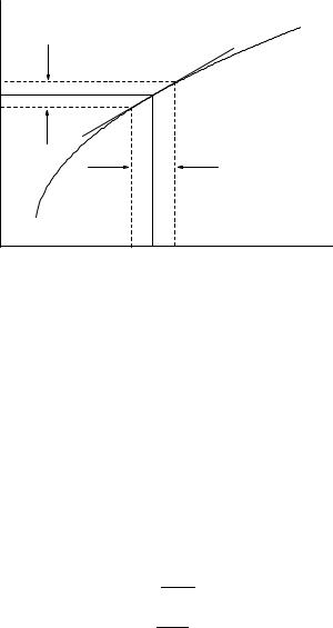
Fig. 4.1. Linear error propagation.
(δy)2 = h(y − ym)2i
≈ h(y(xm) + y′(xm)Δx − ym)2i
=y′2(xm)h(Δx)2i
=y′2(xm)(δx)2 , δy = |y′(xm)|δx .
This result also could have been red o directly from Fig. 4.1.
Examples of the linear propagation of errors for some simple functions are compiled below:
Function : |
Relation between errors : |
|||||||||
y = axn |
|
|
δy |
|
= |
|
|n|δx |
|
||
|
y |
| |
x |
|||||||
|
|
| |
|
| | |
|
|
||||
y = a ln(bx) |
|
δy = |
|a|δx |
|
|
|||||
|
|
|
|
|
|
|
x |
|||
|
|
|
δy |
|
| | |
|
|
|||
y = aebx |
|
= |
|b|δx |
|||||||
|
|
|
||||||||
|
|y| |
|||||||||
y = tan x |
|
δy |
|
= |
|
|
δx |
|
||
|
|y| |
|
| cos x sin x| |
|||||||
4.3.2 Error of a Function of Several Measured Quantities
Most physical measurements depend on several input quantities and their uncertainties. For example, a velocity measurement v = s/t based on the measurements of length and time has an associated error which obviously depends on the errors of both s and t.
Let us first consider a function y(x1, x2) of only two measured quantities with values x1m, x2m and errors δx1, δx2. With the Taylor expansion

96 |
4 Measurement errors |
|
|
|
|
|
|
|
y = y(x1m, x2m) + |
∂y |
(x1m, x2m)Δx1 |
+ |
∂y |
(x1m, x2m)Δx2 |
+ · · · |
|
|
|
|||||
|
∂x1 |
∂x2 |
we get as above to lowest order:
ym = hy(x1, x2)i = y(x1m, x2m)
and |
|
|
|
|
|
|
|
|
|
|
|
|
|
|
|
|
|
|
|
|
|
|
|
(δy)2 = h(Δy)2i |
|
|
|
|
|
|
|
|
|
|
|
|
|
|
|
|
|
|
|
|
|
||
|
∂y |
2 |
|
2 |
|
|
∂y |
2 |
2 |
|
|
|
|
∂y |
|
∂y |
|
|
|||||
= ( |
|
) h(Δx1) |
i + ( |
|
) h(Δx2) |
i + 2( |
|
|
)( |
|
)hΔx1 |
Δx2i |
|
||||||||||
∂x1 |
∂x2 |
∂x1 |
∂x2 |
|
|||||||||||||||||||
|
∂y |
2 |
2 |
|
|
∂y |
2 |
2 |
|
|
|
∂y |
|
|
∂y |
|
|
|
|
(4.5) |
|||
= ( |
|
) (δx1) |
|
+ ( |
|
|
) (δx2) |
+ 2( |
|
)( |
|
|
)R12δx1δx2 , |
||||||||||
∂x1 |
|
∂x2 |
∂x1 |
∂x2 |
|||||||||||||||||||
|
|
|
|
|
|
|
|
|
|
|
|
|
|
|
|
|
|
||||||
with the correlation coe cient |
|
|
|
|
|
|
|
|
|
|
|
|
|
|
|
|
|
|
|
||||
|
|
|
|
|
R12 |
= |
hΔx1Δx2i |
. |
|
|
|
|
|
|
|
|
|
||||||
|
|
|
|
|
|
|
|
|
|
δx1δx2 |
|
|
|
|
|
|
|
|
|
|
|
|
|
In most cases the quantities x1 and x2 are uncorrelated. Then the relation (4.5) simplifies with R12 = 0 to
2 |
∂y 2 |
2 |
∂y 2 |
2 |
||
(δy) = ( |
|
) (δx1) + ( |
|
) (δx2) . |
||
∂x1 |
∂x2 |
|||||
If the function is a product of independent quantities, it is convenient to use relative errors as indicated in the following example:
z |
z |
= xnym , |
+ |
m y |
. |
||||||
|
|
= |
n x |
|
|||||||
|
δz |
|
2 |
|
|
δx |
2 |
|
|
δy |
2 |
It is not di cult to generalize our results to functions y(x1, .., xN ) of N measured quantities. We obtain
|
N |
|
|
|
|
|
|
Rij δxiδxj |
|
|
|
|
|
X |
|
∂y |
∂y |
|
|
|
|
||||
(δy)2 |
= i,j=1 |
∂xi |
|
∂xj |
|
|
|
|
||||
|
N |
|
|
|
|
|
|
N |
|
|
|
Rij δxiδxj |
|
X |
∂y |
|
|
6X |
∂y ∂y |
||||||
|
= i=1 |
|
)2 |
(δxi)2 + i=j=1 |
|
|
|
|||||
|
∂xi |
∂xi ∂xj |
||||||||||
with the correlation coe cient
Rij = hΔxiΔxj i ,
δxiδxj
Rij = Rji ,
Rii = 1 .