

vstatmp_engl
.pdf1.5 Outline of this Book |
7 |
-Very useful especially for the solution of numerical problems is a book by Blobel and Lohrman “Statistische und numerische Methoden der Datenanalyse” [8] written in German.
-Other useful books written by particle physicists are found in Refs. [9, 10, 11, 12]. The books by Roe and Barlow are more conventional while Cowan and D’Agostini favor a moderate Bayesian view.
-Modern techniques of statistical data analysis are presented in a book written by professional statisticians for non-professional users, Hastie et al. “The Elements of Statistical Learning”[13]
-A modern professional treatment of Bayesian statistics is the textbook by Box and Tiao “Bayesian Inference in Statistical Analysis” [14].
The interested reader will find work on the foundations of statistics, on basic principles and on the standard theory in the following books:
-Fisher’s book [15] “Statistical Method, Experimental Design and Scientific Inference” provides an interesting overview of his complete work.
-Edward’s book “Likelihood” [16] stresses the importance of the likelihood function, contains many useful references and the history of the Likelihood Principle.
-Many basic considerations and a collection of personal contributions from a moderate Bayesian view are contained in the book “Good Thinking” by Good [17]. A collection of work by Savage [18], presents a more extreme Baysian point of view.
-Somewhat old fashioned textbooks of Bayesian statistic which are of historical interest are the books of Je reys [19] and Savage [20].
Recent statistical work by particle physicists and astrophysicists can be found in the proceedings of the PHYSTAT Conferences [21] held during the past few years. Many interesting and well written articles can be found also in the internet.
This personal selection of literature is obviously in no way exhaustive.

2
Basic Probability Relations
2.1 Random Events and Variables
Events are processes or facts that are characterized by a specific property, like obtaining a “3” with a dice. A goal in a soccer play or the existence of fish in a lake are events. Events can also be complex facts like rolling two times a dice with the results three and five or the occurrence of a certain mean value in a series of measurements or the estimate of the parameter of a theory. There are elementary events, which mutually exclude each other but also events that correspond to a class of elementary events, like the result greater than three when throwing a dice. We are concerned with random events which emerge from a stochastic process as already introduced above.
When we consider several events, then there are events which exclude each other and events which are compatible. We stick to our standard example dice. The elementary events three and five exclude each other, the events greater than two and five are of course compatible. An other common example: We select an object from a bag containing blue and red cubes and spheres. Here the events sphere and cube exclude each other, the events sphere and red may be compatible.
The event A is called the complement of event A if either event A or event A applies, but not both at the same time (exclusive or ). Complementary to the event three in the dice example is the event less than three or larger than three (inclusive or ). Complementary to the event red sphere is the event cube or blue sphere.
The event consisting of the fact that an arbitrary event out of all possible events applies, is called the certain event. We denote it with Ω. The complementary event is the impossible event, that none of all considered events applies: It is denoted with, thus = Ω.
Some further definitions are useful: Definition 1: A B means A or B.
The event A B has the attributes of event A or event B or those of both A and B (inclusive or ). (The attribute cube red corresponds to the complementary event
blue sphere.)
Definition 2: A ∩ B means A and B.

10 2 Basic Probability Relations
The event A ∩ B has the attributes of event A as well as those of event B. (The attribute cube ∩ red corresponds to red cube.) If A ∩ B = , then A, B mutually exclude each other.
Definition 3: A B means that A implies B.
It is equivalent to both A B = B and A ∩ B = A. From these definitions follow the trivial relations
A A = Ω , A ∩ A = , |
|
and |
|
A Ω . |
(2.1) |
For any A, B we have
A B = A ∩ B , A ∩ B = A B .
To the random event A we associate the probability P {A} as discussed above. In all practical cases random events can be identified with a variable, the random variable or variate. Examples for variates are the decay time in particle decay, the number of cosmic muons penetrating a body in a fixed time interval and measurement errors. When the random events involve values that cannot be ordered, like shapes or colors, then they can be associated with classes or categorical variates.
2.2 Probability Axioms and Theorems
2.2.1 Axioms |
|
|
|
|
|
|
|
The assignment of probabilities P |
{ |
A |
} |
to members A, B, C, ... of a set of events |
|||
|
|
|
|
|
|
||
has to satisfy the following axioms |
|
. Only then the rules of probability theory are |
|||||
|
|
|
1 |
|
|
|
|
applicable. |
|
|
|
|
|
|
|
• |
Axiom 1 |
0 ≤ P {A} |
|
|
|
|
|
|
The probability of an event is a positive real number. |
||||||
• |
Axiom 2 |
P {Ω} = 1 |
|
|
|
|
|
|
The probability of the certain event is one. |
||||||
•Axiom 3 P {A B} = P {A} + P {B} if A ∩ B =
The probability that A or B applies is equal to the sum of the probabilities that A or that B applies, if the events A and B are mutually exclusive.
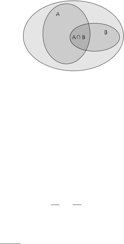
These axioms and definitions imply the following theorems whose validity is rather obvious. They can be illustrated with so-called Venn diagrams, Fig. 2.1. There the areas of the ellipses and their intersection are proportional to the probabilities.
P {A} = 1 − P {A} , P { } = 0 ,
P {A B} = P {A} + P {B} − P {A ∩ B} ,
if A B |
P {A} ≤ P {B} . |
(2.2) |
1They are called Kolmogorov axioms, after the Russian mathematician A. N. Kolmogorov (1903-1987).

2.2 Probability Axioms and Theorems |
11 |
Relation (2.1) together with (2.2) and axioms 1, 2 imply 0 ≤ P {A} ≤ 1. For arbitrary events we have
P {A B} ≥ P {A} , P {B} ; P {A ∩ B} ≤ P {A} , P {B} .
If all events with the attribute A possess also the attribute B, A B, then we have
P {A ∩ B} = P {A}, and P {A B} = P {B}.
2.2.2 Conditional Probability, Independence, and Bayes’ Theorem
In the following we need two further definitions:
Definition: P {A | B} is the conditional probability of event A under the condition that B applies. It is given, as is obvious from Fig. 2.1, by:
P |
{ |
A |
| |
B |
} |
= |
P {A ∩ B} |
, |
P |
{ |
B |
= 0 . |
(2.3) |
|||
|
|
|
|
P |
{ |
B |
} |
|
|
|
} 6 |
|
||||
|
|
|
|
|
|
|
|
|
|
|
|
|
|
|
||
A conditional probability is, for example, the probability to find a sphere among the red objects. The notation A | B expresses that B is considered as fixed, while A is the random event to which the probability refers. Contrary to P {A}, which refers to arbitrary events A, we require that also B is valid and therefore P {A ∩ B} is normalized to P {B}.
Among the events A | B the event A = B is the certain event, thus P {B | B} = 1. More generally, from definition 3 of the last section and (2.3) follows P {A|B} = 1 if B implies A:
B A A ∩ B = B P {A|B} = 1 .
Definition: If P {A ∩ B} = P {A} × P {B}, the events A and B (more precisely: the probabilities for their occurrence) are independent.
From (2.3) then follows P {A | B} = P {A}, i.e. the conditioning on B is irrelevant for the probability of A. Likewise P {B | A} = P {B}.
In Relation (2.3) we can exchange A and B and thus P {A | B}P {B} = P {A ∩
B} = P {B | A}P {A} and we obtain the famous Bayes’ theorem: |
|
P {A | B}P {B} = P {B | A}P {A} . |
(2.4) |
Bayes’ theorem is frequently used to relate the conditional probabilities P {A | B} and P {B | A}, and, as we will see, is of some relevance in parameter inference.
The following simple example illustrates some of our definitions. It assumes that each of the considered events is composed of a certain number of elementary events which mutually exclude each other and which because of symmetry arguments all have the same probability.
Example 2. Card game, independent events
The following table summarizes some probabilities for randomly selected cards from a card set consisting of 32 cards and 4 colors.
12 2 Basic Probability Relations
Fig. 2.1. Venn diagram.
P {king}: |
4/32 |
= 1/8 |
(prob. for king) |
|
P {heart}: |
1/4 |
· |
|
(prob. for heart) |
P {heart ∩ king}: 1/8 |
1/4 = 1/32 |
(prob. for heart king) |
||
P {heart king}: 1/8 |
+ 1/4 − 1/32 = 11/32 (prob. for heart or king) |
|||
P {heart | king}: |
1/4 |
|
|
(prob. for heart if king) |
The probabilities P {heart} and P {heart | king} are equal as required from the independence of the events A and B.
The following example illustrates how we make use of independence.
Example 3. Random coincidences, measuring the e ciency of a counter
When we want to measure the e ciency of a particle counter (1), we combine it with a second counter (2) in such a way that a particle beam crosses both detectors. We record the number of events n1, n2 in the two counters and in addition the number of coincidences n1∩2. The corresponding e ciencies relate these numbers2 to the unknown number of particles n crossing the detectors.
n1 = ε1n , n2 = ε2n , n1∩2 = ε1∩2n .
For independent counting e ciencies we have ε1∩2 = ε1ε2 and we get
ε1 |
= |
n1∩2 |
, ε2 |
= |
n1∩2 |
, n = |
n1n2 |
. |
|
||||||||
|
|
n2 |
|
n1 |
|
n1∩2 |
||
This scheme is used in many analog situations.
Bayes’ theorem is applied in the next two examples, where the attributes are not independent.
Example 4. Bayes’ theorem, fraction of women among students
2Here we ignore the statistical fluctuations of the observations.

2.2 Probability Axioms and Theorems |
13 |
From the proportion of students and women in the population and the fraction of students among women we compute the fraction of women among students:
P {A} |
= 0.02 |
(fraction of students in the population) |
P {B} |
= 0.5 |
(fraction of women in the population) |
P {A | B} = 0.018 |
(fraction of students among women) |
|
P {B | A} =? |
(fraction of women among students) |
|
The dependence of the events A and B manifests itself in the di erence of P {A} and P {A | B}. Applying Bayes’ theorem we obtain
P {B | A} = P {A | B}P {B} P {A}
= 0.018 · 0.5 = 0.45 . 0.02
About 45% of the students are women.
Example 5. Bayes’ theorem, beauty filter
The probability P {A} that beauty quark production occurs in a colliding beam reaction be 0.0001. A filter program selects beauty reactions A with e ciency P {b | A} = 0.98 and the probability that it falsely assumes that beauty is present if it is not, be P {b | A} = 0.01. What is the probability P {A | b} to have genuine beauty production in a selected event? To solve the problem, first the probability P {b} that a random event is selected has to be evaluated,
|
|
|
|
|
|
|
|
|
|
A |
|
|
|
|
|
P {b} = P {b} P {A | b} + P {A | b} |
|
|
|
||||||||||||
|
{ |
|
| } |
{ } |
{ |
|
|
| |
|
|
} |
|
|
|
|
= P |
b |
b |
|
|
P |
{ } |
|||||||||
|
A P |
A + P |
|
|
|
|
|
|
A |
||||||
where the bracket in the first line is equal to 1. In the second line Bayes’ theorem is applied. Applying it once more, we get
P {A | b} = P {b | A}P {A}
P {b}
P {b | A}P {A}
=
P {b | A}P {A} + P {b | A}P {A}
0.98 · 0.0001 = 0.98 · 0.0001 + 0.01 · 0.9999 = 0.0097 .
About 1% of the selected events corresponds to b quark production.
Bayes’ theorem is rather trivial, thus the results of the last two examples could have easily been written down without referring to it.
3
Probability Distributions and their Properties
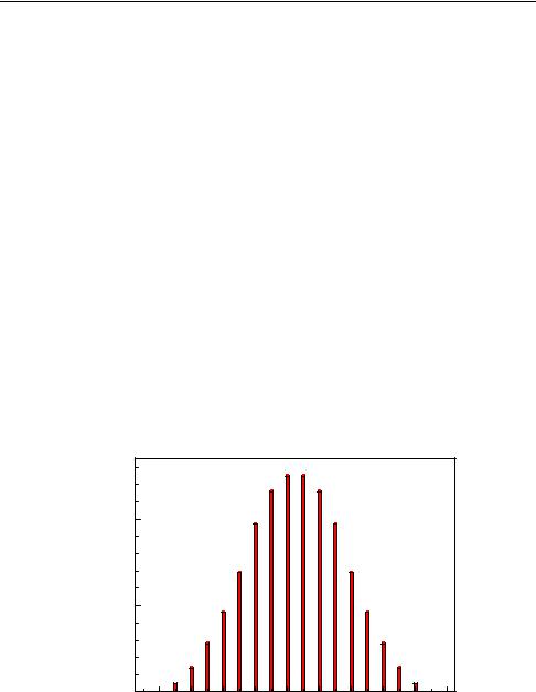
A probability distribution assigns probabilities to random variables. As an example we show in Fig. 3.1 the distribution of the sum s of the points obtained by throwing three ideal dice. Altogether there are 63 = 216 di erent combinations. The random variable s takes values between 3 and 18 with di erent probabilities. The sum s = 6, for instance, can be realized in 10 di erent ways, all of which are equally probable. Therefore the probability for s = 6 is P {s = 6} = 10/216 ≈ 4.6 %. The distribution is symmetric with respect to its mean value 10.5. It is restricted to discrete values of s, namely natural numbers.
In our example the variate is discrete. In other cases the random variables are continuous. Then the probability for any fixed value is zero, we have to describe the distribution by a probability density and we obtain a finite probability when we integrate the density over a certain interval.
probability
0.10
0.05
0.00 |
2 |
4 |
6 |
8 |
10 |
12 |
14 |
16 |
18 |
20 |
|
sum
Fig. 3.1. Probability distribution of the sum of the points of three dice.

16 3 Probability Distributions and their Properties
3.1 Definition of Probability Distributions
We define a distribution function, also called cumulative or integral distribution function, F (t), which specifies the probability P to find a value of x smaller than t:
F (t) = P {x < t} , with − ∞ < t < ∞ .
The probability axioms require the following properties of the distribution function:
a)F (t) is a non-decreasing function of t ,
b)F (−∞) = 0 ,
c)F (∞) = 1 .
We distinguish between
•Discrete distributions (Fig. 3.2)
•Continuous distributions (Fig. 3.3)
3.1.1 Discrete Distributions
If not specified di erently, we assume in the following that discrete distributions assign probabilities to an enumerable set of di erent events, which are characterized by an ordered, real variate xi, with i = 1, . . . , N, where N may be finite or infinite. The probabilities p(xi) to observe the values xi satisfy the normalization condition:
XN
p(xi) = 1 .
i=1
It is defined by
p(xi) = P {x = xi} = F (xi + ǫ) − F (xi − ǫ) ,
with ǫ positive and smaller than the distance to neighboring variate values.
Example 6. Discrete probability distribution (dice)
For a fair die, the probability to throw a certain number k is just one-sixth: p(k) = 1/6 for k = 1, 2, 3, 4, 5, 6.
It is possible to treat discrete distributions with the help of Dirac’s δ-function like continuous ones. Therefore we will often consider only the case of continuous variates.
3.1.2 Continuous Distributions
We replace the discrete probability distribution by a probability density1 f(x), abbreviated as p.d.f. (probability density function). It is defined as follows:
1We will, however, use the notations probability distribution and distribution for discrete as well as for continuous distributions.