

vstatmp_engl
.pdf3.1 Definition of Probability Distributions |
17 |
0.2
P(x)
0.1
0.0
x
1.0
F(x)
0.5
0.0
x
Fig. 3.2. Discrete probability distribution and distribution function.
f(x) = |
dF (x) |
. |
(3.1) |
|
|||
|
dx |
|
|
Remark that the p.d.f. is defined in the full range −∞ < x < ∞. It may be zero in certain regions.
It has the following properties:
a)f(−∞) = f(+∞) = 0 ,
b)R−∞∞ f(x)dx = 1 .
The probability P {x1 ≤ x ≤ x2} to find the random variable x in the interval [x1, x2] is given by
Z x2
P {x1 ≤ x ≤ x2} = F (x2) − F (x1) = |
f(x)dx . |
x1
We will discuss specific distributions in Sect. 3.6 but we introduce two common distributions already here. They will serve us as examples in the following sections.
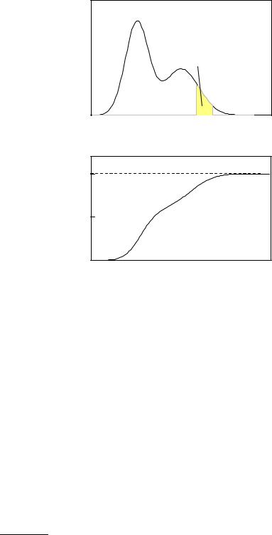
Example 7. Probability density of an exponential distribution
The decay time t of an instable particles follows an exponential distribution with the p.d.f.
18 3 Probability Distributions and their Properties
f(x) |
|
P(x |
< x < x ) |
|
|
|
1 |
2 |
|
|
|
x |
x |
|
|
x |
1 |
2 |
|
|
|
|
|
|
1.0 |
|
|
|
|
F(x) |
|
|
|
|
0.5 |
|
|
|
|
0.0 |
|
|
|
|
|
x |
|
|
|
Fig. 3.3. Probability density and distribution function of a continuous distribution.
f(t) |
≡ |
f(t |
λ) = λe−λt |
for t |
≥ |
0 , |
(3.2) |
|
| |
|
|
|
|
where the parameter2 λ > 0, the decay constant, is the inverse of the mean lifetime τ = 1/λ. The probability density and the distribution function
Z t
F (t) = f(t′)dt′ = 1 − e−λt
−∞
are shown in Fig. 3.4. The probability of observing a lifetime longer than τ is
P {t > τ} = F (∞) − F (τ) = e−1 .
Example 8. Probability density of the normal distribution
An oxygen atom is drifting in argon gas, driven by thermal scattering. It starts at the origin. After a certain time its position is (x, y, z). Each projec-
2We use the bar | to separate random variables (x, t) from parameters (λ) which specify the distribution. This notation will be discussed below in Chap. 6, Sect. 6.3.

3.1 Definition of Probability Distributions |
19 |
0.50 |
|
|
|
|
|
|
f(x) |
|
f(x)= |
- |
x |
|
|
0.25 |
|
e |
|
|
|
|
|
|
|
|
|
|
|
0.000 |
2 |
4 |
|
6 |
8 |
10 |
|
|
|
x |
|
|
|
1.0 |
|
|
|
|
|
|
F(x) |
|
|
|
- |
x |
|
0.5 |
|
F(x)=1-e |
|
|
||
|
|
|
|
|
|
|
0.00 |
2 |
4 |
|
6 |
8 |
10 |
|
|
|
x |
|
|
|
Fig. 3.4. Probability density and distribution function of an exponential distribution.
tion, for instance x, has approximately a normal distribution (see Fig. 3.5), also called Gauss distribution3
f(x) = N(x|0, s) ,
1 |
|
2 |
2 |
(3.3) |
||
N(x|x0, s) = |
√ |
|
|
e−(x−x0) |
/(2s ) . |
|
2πs |
||||||
The width constant s is, as will be shown later, proportional to the square root of the number of scattering processes or the square root of time. When we descent by the factor 1/√e from the maximum, the full width is just 2s. A statistical drift motion, or more generally a random walk, is met frequently in science and also in every day life. The normal distribution also describes approximately the motion of snow flakes or the erratic movements of a drunkard in the streets.
3In the formula we separate parameters from variates by a bar.

20 3 Probability Distributions and their Properties
0.3
|
0.2 |
f(x) |
2s |
|
|
|
0.1 |
0.0-6 |
-4 |
-2 |
0 |
2 |
4 |
6 |
x
Fig. 3.5. Normal distribution.
3.1.3 Empirical Distributions
Many processes are too complex or not well enough understood to be described by a distribution in form of a simple algebraic formula. In these cases it may be useful to approximate the underlying distribution using an experimental data sample. The simplest way to do this, is to histogram the observations and to normalize the frequency histogram. More sophisticated methods of probability density estimation will be sketched in Chap. 12. The quality of the approximation depends of course on the available number of observations.
3.2 Expected Values
In this section we will consider some general characteristic quantities of distributions, like mean value, width, and asymmetry or skewness. Before introducing the calculation methods, we turn to the general concept of the expected value.
The expected value E(u) of a quantity u(x), which depends on the random variable x, can be obtained by collecting infinitely many random values xi from the distribution f(x), calculating ui = u(xi), and then averaging over these values. Obviously, we have to assume the existence of such a limiting value.
In quantum mechanics, expected values of physical quantities are the main results of theoretical calculations and experimental investigations, and provide the connection to classical mechanics. Also in statistical mechanics and thermodynamics the calculation of expected values is frequently needed. We can, for instance, calculate
3.2 Expected Values |
21 |
from the velocity distribution of gas molecules the expected value of their kinetic energy, that means essentially their temperature. In probability theory and statistics expected values play a central role.
3.2.1 Definition and Properties of the Expected Value
Definition:
|
∞ |
|
|
|
Xi |
(discrete distribution) , |
(3.4) |
E(u(x)) = |
u(xi)p(xi) |
||
|
=1 |
|
|
|
∞ |
|
|
E(u(x)) = Z−∞ u(x)f(x) dx (continuous distribution) . |
(3.5) |
||
Here and in what follows, we assume the existence of integrals and sums. This condition restricts the choice of the allowed functions u, p, f.
From the definition of the expected value follow the relations (c is a constant, u, v are functions of x):
E(c) = c, |
(3.6) |
E(E(u)) = E(u), |
(3.7) |
E(u + v) = E(u) + E(v), |
(3.8) |
E(cu) = cE(u) . |
(3.9) |
They characterize E as a linear functional.
For independent (see also Chap. 2 and Sect. 3.5) variates x, y the following important relation holds:
E (u(x)v(y)) = E(u)E(v) . |
(3.10) |
Often expected values are denoted by angular brackets:
E(u) ≡ hui .
Sometimes this simplifies the appearance of the formulas. We will use both notations.
In case of a nonlinear function u(x), its expected value di ers, in general, from its value at the argument hxi:
hui 6= u(hxi) .
Example 9. Relation between the expected values of the track momentum and of its curvature
In tracking detectors the momentum p of a charged particle is usually determined from the curvature ρ in a magnetic field, p(ρ) = c/ρ. Here hp(ρ)i > p(hρi) = c/hρi. In fact the momentum determined from the curvature is biased to large values. More generally, if u(x) is the inverse of a positive function v(x), its expected value is always greater than (or equal to) the inverse expected value of v:
hui = h1/vi ≥ 1/ hvi ,

22 3 Probability Distributions and their Properties
where equality is only possible in the degenerate case of a one-point distribution f(x) = δ(x − c).
To show this assertion, we define an inner product of two positive functions g(x), h(x) of a random variable x with p.d.f. f(x):
Z
(g, h) = g(x)h(x)f(x)dx
and apply the Cauchy–Schwarz inequality
(g, h)2 ≤ (g, g)(h, h)
p p
to g(x) = u(x) and h(x) = 1/ u(x), giving
hui h1/ui ≥ 1 .
The equality requires g h, or f(x) = δ(x − c).
3.2.2 Mean Value
The expected value of the variate x is also called the mean value. It can be visualized as the center of gravity of the distribution. Usually it is denoted by the Greek letter µ. Both names, mean value, and expected value4 of the corresponding distribution are used synonymously.
Definition:
|
≡ hxi = µ = |
∞ |
|
E(x) |
i=1 xip(xi) (discrete distribution) , |
||
|
≡ h i |
R−∞ |
|
E(x) |
x |
= µ = |
∞ |
P x f(x) dx (continuous distribution) . |
|||
The mean value of the exponential distribution (3.2) is
Z ∞
hti = λte−λt dt = 1/λ = τ .
0
We will distinguish hxi from the average value of a sample, consisting of a finite number N of variate values, x1, . . . , xN , which will be denoted by x:
1 X
x = N i xi .
It is called sample mean. It is a random variable and has the expected value
hxi = |
1 |
Xi |
hxii = hxi , |
N |
as follows from (3.8), (3.9).
4The notation expected value may be somewhat misleading, as the probability to obtain it can be zero (see the example “dice” in Sect. 3.2.7).
3.2 Expected Values |
23 |
3.2.3 Variance
The variance σ2 measures the spread of a distribution, defined as the mean quadratic deviation of the variate from its mean value. Usually, we want to know not only the mean value of a stochastic quantity, but require also information on the dispersion of the individual random values relative to it. When we buy a laser, we are of course interested in its mean energy per pulse, but also in the variation of the single energies around that mean value. The mean value alone does not provide information about the shape of a distribution. The mean height with respect to sea level of Switzerland is about 700 m, but this alone does not say much about the beauty of that country, which, to a large degree, depends on the spread of the height distribution.
The square root σ of the variance is called standard deviation and is the standard measure of stochastic uncertainties.
A mechanical analogy to the variance is the moment of inertia for a mass distribution along the x-axis for a total mass equal to unity.
Definition: |
(x − µ)2 . |
var(x) = σ2 = E |
|
From this definition follows immediately |
|
var(cx) = c2var(x) ,
and σ/µ is independent of the scale of x.
Very useful is the following expression for the variance which is easily derived from its definition and (3.8), (3.9):
σ2 = E(x2 − 2xµ + µ2)
=E(x2) − 2µ2 + µ2
=E(x2) − µ2.
Sometimes this is written more conveniently as
σ2 = hx2i − hxi2 = hx2i − µ2 . |
(3.11) |
In analogy to Steiner’s theorem for moments of inertia, we have
h(x − a)2i = h(x − µ)2i + h(µ − a)2i
= σ2 + (µ − a)2 ,
implying (3.11) for a = 0.
The variance is invariant against a translation of the distribution by a:
x → x + a , µ → µ + a σ2 → σ2 .
Variance of a Sum of Random Numbers
Let us calculate the variance σ2 for the distribution of the sum x of two independent random numbers x1 and x2, which follow di erent distributions with mean values µ1, µ2 and variances σ12, σ22:

243 Probability Distributions and their Properties x = x1 + x2,
σ2 = h(x − hxi)2i
=h((x1 − µ1) + (x2 − µ2))2i
=h(x1 − µ1)2 + (x2 − µ2)2 + 2(x1 − µ1)(x2 − µ2)i
=h(x1 − µ1)2i + h(x2 − µ2)2i + 2hx1 − µ1ihx2 − µ2i
=σ12 + σ22 .
In the fourth step the independence of the variates (3.10) was used.
This result is important for all kinds of error estimation. For a sum of two independent measurements, their standard deviations add quadratically. We can generalize the last relation to a sum x = P xi of N variates or measurements:
|
N |
|
σ2 = |
Xi |
(3.12) |
σ2 . |
||
|
i |
|
|
=1 |
|
Example 10. Variance of the convolution of two distributions
We consider a quantity x with the p.d.f. g(x) with variance σg2 which is measured with a device which produces a smearing with a p.d.f. h(y) with variance σh2 . We want to know the variance of the “smeared” value x′ = x+ y. According to 3.12, this is the sum of the variances of the two p.d.f.s:
σ2 = σg2 + σh2 .
Variance of the Sample Mean of Independent Identically Distributed
Variates
From the last relation we obtain the variance σx2 of the sample mean x from N independent random numbers xi, which all follow the same distribution5 f(x), with expected value µ and variance σ2:
XN
x = xi/N ,
i=1
var(Nx) = N2 var(x) = Nσ2 ,
σx = √σ . (3.13)
N
The last two relations (3.12), (3.13) have many applications, for instance in ran-
dom walk, di usion, and error propagation. The root mean square distance reached
√
by a di using molecule after N scatters is proportional to N and therefore also to
√
t, t being the di usion time. The total length of 100 aligned objects, all having the same standard deviation σ of their nominal length, will have a standard deviation of only 10 σ. To a certain degree, random fluctuations compensate each other.
5The usual abbreviation is i.i.d. variates for independent identically distributed.

3.2 Expected Values |
25 |
Width v of a Sample and Variance of the Distribution
Often, as we will see in Chap. 6, a sample is used to estimate the variance σ2 of the underlying distribution. In case the mean value µ is known, we calculate the quantity
vµ2 = N1 X (xi − µ)2
i
which has the correct expected value hvµ2 i = σ2. Usually, however, the true mean value µ is unknown – except perhaps in calibration measurements – and must be estimated from the same sample as is used to derive vµ2 . We then are obliged to use the sample mean x instead of µ and calculate the mean quadratic deviation v2 of the sample values relative to x. In this case the expected value of v2 will depend not only on σ, but also on N. In a first step we find
v2 = |
1 |
Xi |
(xi − |
|
|
)2 |
|
|
|
|
|
|
|
|
|
|
|
|
||||||||||||
|
|
|
x |
|
|
|
|
|
|
|
|
|
|
|
|
|||||||||||||||
|
N |
|
|
|||||||||||||||||||||||||||
|
= |
1 |
Xi |
|
xi2 − 2xi |
|
|
+ |
|
|
2 |
|
|
|||||||||||||||||
|
|
|
|
|
x |
x |
|
|
||||||||||||||||||||||
|
|
N |
|
|
|
|||||||||||||||||||||||||
|
= |
1 |
Xi |
xi2 − |
|
|
2 . |
|
|
|
|
|
|
|
|
|
|
|
||||||||||||
|
|
|
|
x |
|
|
|
|
|
|
|
|
||||||||||||||||||
|
|
N |
|
|
||||||||||||||||||||||||||
To calculate the expected value, we use (3.11) and (3.13), |
|
|
||||||||||||||||||||||||||||
|
|
hx2i = σ2 + µ2 , |
|
|
||||||||||||||||||||||||||
|
|
h |
|
2i = var( |
|
) + h |
|
i2 |
|
|
||||||||||||||||||||
|
x |
x |
x |
|
|
|||||||||||||||||||||||||
|
|
|
|
|
|
= |
|
σ2 |
+ µ2 |
|
|
|
|
|
|
|
|
|
|
|
|
|
||||||||
|
|
|
|
|
|
|
N |
|
|
|
|
|
|
|
|
|
|
|
|
|
||||||||||
|
|
|
|
|
|
|
|
|
|
|
|
|
|
|
|
|
|
|
|
|
|
|
|
|
|
|
|
|
||
and get with (3.14) |
|
|
|
|
|
|
|
|
|
|
|
|
|
|
|
|
|
1 − N |
|
|
||||||||||
hv2i = hx2i − hx2i = σ2 |
, |
|||||||||||||||||||||||||||||
|
|
|
|
|
|
|
|
|
|
|
|
|
|
|
|
|
|
|
1 |
|
|
|
|
|||||||
|
|
N − 1 h |
i |
|
|
|
hP N − 1 |
i |
||||||||||||||||||||||
σ2 |
= |
|
N |
|
v2 |
|
= |
|
|
|
|
|
i (xi − |
x |
)2 |
|
. |
|||||||||||||
|
|
|
|
|
|
|
|
|
|
|
|
|
|
|
||||||||||||||||
(3.14)
(3.15)
The expected value of the mean squared deviation is smaller than the variance of the distribution by a factor of (N − 1)/N.
The relation (3.15) is widely used for the estimation of measurement errors, when several independent measurements are available. The variance σx2 of the sample mean x itself is approximated, according to (3.13), by
− |
|
|
P |
|
− |
|
|
)2 |
|
v2 |
|
= |
i |
(xi − |
x |
. |
|||
N |
1 |
|
N(N |
|
1) |
|
|||
Mean Value and Variance of a Superposition of two Distributions
Frequently a distribution consists of a superposition of elementary distributions. Let us compute the mean µ and variance σ2 of a linear superposition of two distributions
26 3 Probability Distributions and their Properties
f(x) = αf1(x) + βf2(x) , α + β = 1 ,
where f1, f2 may have di erent mean values µ1, µ2 and variances σ12, σ22:
µ= αµ1 + βµ2 ,
σ2 = E (x − E(x))2
=E(x2) − µ2
=αE1(x2) + βE2(x2) − µ2
=α(µ21 + σ12) + β(µ22 + σ22) − µ2
=ασ12 + βσ22 + αβ(µ1 − µ2)2 .
Here, E, E1, E2 denote expected values related to the p.d.f.s f, f1, f2. In the last step the relation α + β = 1 has been used. Of course, the width increases with the distance of the mean values. The result for σ2 could have been guessed by considering the limiting cases, µ1 = µ2, σ1 = σ2 = 0.
3.2.4 Skewness
The skewness coe cient γ1 measures the asymmetry of a distribution with respect to its mean. It is zero for the normal distribution, but quite sizable for the exponential distribution. There it has the value γ1 = 2, see Sect. 3.3.3 below.
Definition: |
h |
i |
|
γ1 = E (x − µ)3 /σ3 .
Similarly to the variance, γ1 can be expressed by expected values of powers of the variate x:
|
= E x − 3 |
|
|
|
|
− |
|
|
|
||||
γ1 |
= E (x − µ)3 |
/σ3 |
|
− |
|
− |
|
||||||
|
|
|
− |
|
|
|
|||||||
|
= |
3 |
− |
|
µx2 + 3µ2x µ3 |
/σ3 |
|
||||||
|
|
|
|
− |
|
. |
|
|
|
µ3 /σ3 |
|||
|
= E(x3) 3µ E(x2) µE(x) |
|
|||||||||||
|
|
E(x3) |
|
3µσ2 |
µ3 |
|
|
|
|
|
|||
|
|
|
|
|
σ3 |
|
|
|
|
|
|
|
|
The skewness coe cient is defined in such a way that it satisfies the requirement of invariance under translation and dilatation of the distribution. Its square is usually denoted by β1 = γ12.
3.2.5 Kurtosis (Excess)
A fourth parameter, the kurtosis β2, measures the tails of a distribution.
Definition: |
|
|
|
|
β2 = E (x |
|
µ)4 |
/σ4 . |
|
A kurtosis coe cient or excess γ2, |
|
− |
|
|
γ2 = β2 − 3 ,
is defined such that it is equal to zero for the normal distribution which is used as a reference. (see Sect. 3.6.5).