

vstatmp_engl
.pdf3.5 |
Multivariate Probability Densities |
47 |
|||
g(u, v) du dv = f(x, y) dx dy , |
|
||||
|
|
∂(x, y) |
|
|
|
|
|
|
|
|
|
g(u, v) = f(x, y) |
|
∂(u, v) |
|
, |
|
|
|
|
|
|
|
with the Jacobian determinant replacing the di erential quotient dx/du.
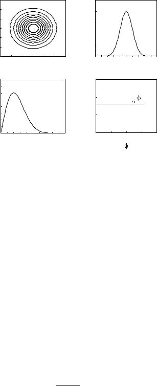
Example 29. Transformation of a normal distribution from cartesian into polar coordinates
A two-dimensional normal distribution
f(x, y) = 21π e−(x2+y2)/2
is to be transformed into polar coordinates
x = r cos ϕ , y = r sin ϕ .
The Jacobian is
∂(x, y) = r .
∂(r, ϕ)
We get |
|
1 |
|
|
|
|
g(r, ϕ) = |
re−r2/2 |
|||||
|
||||||
|
|
2π |
||||
with the marginal distributions |
|
|
|
|
|
|
gr = Z 2π g(r, ϕ) dϕ = re−r2/2 , |
||||||
0 |
|
|
|
|
|
|
∞ |
|
1 |
|
|||
gϕ = Z0 |
g(r, ϕ) dr = |
|
. |
|||
2π |
||||||
The joined distribution factorizes into its marginal distributions (Fig. 3.13). Not only x, y, but also r, ϕ are independent.
3.5.4 Reduction of the Number of Variables
Frequently, we are faced with the problem to find from a given joined distribution f(x, y) the distribution g(u) of a dependent random variable u(x, y). We can reduce it to that of a usual transformation, by inventing a second variable v = v(x, y), performing the transformation f(x, y) −→ h(u, v) and, finally, by calculating the marginal distribution in u,
Z ∞
g(u) = |
h(u, v) dv . |
−∞
In most cases, the choice v = x is suitable. More formally, we might use the equivalent reduction formula
Z ∞
g(u) = |
f(x, y)δ (u − u(x, y)) dx dy . |
(3.37) |
−∞
48 3 Probability Distributions and their Properties
2 |
a) |
|
|
|
|
|
y 0 |
|
|
|
|
|
|
-2 |
|
|
|
|
|
|
|
-2 |
|
0 |
x |
2 |
|
|
|
|
|
|
|
|
0.8 |
c) |
|
|
|
|
|
0.6 |
|
g (r) |
|
|
|
|
|
|
|
|
|
||
0.4 |
|
|
r |
|
|
|
|
|
|
|
|
|
|
0.2 |
|
|
|
|
|
|
0.00 |
1 |
2 |
3 |
|
4 |
5 |
|
|
|
r |
|
|
|
0.4 |
b) |
|
f (x), f (y) |
||
|
|
x |
y |
|
|
0.2 |
|
|
|
|
|
0.0 |
-4 |
-2 |
0 |
2 |
4 |
|
|||||
|
|
|
|
|
x, y |
0.3 |
d) |
|
|
|
0.2 |
|
g ( |
) |
|
0.1 |
|
|
|
|
0.00 |
2 |
4 |
6 |
8 |
Fig. 3.13. Transformation of a two-dimensional normal distribution of cartesian coordinates into the distribution of polar coordinates: (a) lines of constant probability; b) cartesian marginal distributions; c), d) marginal distributions of the polar coordinates.
For the distribution of a sum u = x + y of two independent variates x, y, i.e. f(x, y) = fx(x)fy (y), after integration over y follows
Z Z
g(u) = f(x, u − x) dx = fx(x)fy (u − x) dx .
This is called the convolution integral or convolution product of fx and fy.
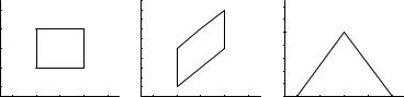
Example 30. Distribution of the di erence of two digitally measured times The true times t1, t2 are taken to follow a uniform distribution
f(t1 |
, t2) = |
1/Delta2 for |
| |
t1 |
− |
T1 |
, |t2 − T2| < Δ/2 |
|
|
0 |
|
|
| else |
around the readings T1, T2. We are interested in the probability density of the di erence t = t1−t2. To simplify the notation, we choose the case T1 = T2 = 0 and = 2 (Fig. 3.14). First we transform the variables according to
t = t1 − t2 , t1 = t1
with the Jacobian
∂(t1, t2) = 1 . ∂(t1, t)
The new distribution is also uniform:
3.5 Multivariate Probability Densities |
49 |
t |
2 |
|
|
|
|
|
t |
2 |
|
|
|
|
|
g(t) |
|
|
|
|
|
|
2 |
1 |
|
|
|
|
|
2 |
1 |
|
|
|
|
|
0.5 |
|
|
|
|
|
|
|
0 |
|
|
|
|
|
|
0 |
|
|
|
|
|
|
|
|
|
|
|
|
|
-1 |
|
|
|
|
|
|
-1 |
|
|
|
|
|
|
|
|
|
|
|
|
|
-2 |
|
|
|
|
|
|
-2 |
|
|
|
|
|
0.0 |
|
|
|
|
|
|
|
-2 |
-1 |
0 |
t |
1 |
2 |
|
-2 |
-1 |
0 |
t |
1 |
2 |
-2 |
-1 |
0 |
t |
1 |
2 |
|
|
|
|
|
|
|
|
|
|
|
|
|
|
|
|
|
|
|
|||
|
|
|
|
1 |
|
|
|
|
|
|
1 |
|
|
|
|
|
|
|
|
Fig. 3.14. Distribution of the di erence t between two times t1 and t2 which have both clock readings equal to zero.
h(t1, t) = f(t1, t2) = 1/Δ2 ,
and has the boundaries shown in Fig. 3.14. The form of the marginal distribution is found by integration over t1, or directly by reading it o from the figure:
|
|
( |
t − T + |
)/Δ2 for t − T < 0 |
|||
g(t) = |
( |
|
t + T + |
)/Δ2 for 0 < t |
|
T |
|
|
|
0− |
|
else . |
− |
|
|
|
|
|
|
||||
where T = T1 − T2 now for arbitrary values of T1 and T2.
Example 31. Distribution of the transverse momentum squared of particle tracks
The projections of the momenta are assumed to be independently normally distributed,
|
f(px, py) = |
|
1 |
|
|
e−(px2 +py2 )/(2s2) , |
||||||||||||||
|
2πs2 |
|||||||||||||||||||
|
|
|
|
|
|
|
|
|
|
|
|
|
|
|||||||
with equal variances |
p2 |
= |
|
|
p2 |
|
|
|
|
= s2. For the transverse momentum |
||||||||||
|
2 |
x |
|
|
|
|
y |
|
|
|
|
|
|
|
|
|
|
|
|
|
squared we set q = p |
|
|
|
|
|
|
|
|
|
|
|
|
|
|
|
|
|
|||
tributions into polar coordinates |
|
|
|
|
|
|
|
|
|
|
|
|
|
|
|
|||||
|
|
|
px = √ |
|
cos ϕ , |
|||||||||||||||
|
|
|
q |
|||||||||||||||||
|
|
|
py = √ |
|
sin ϕ |
|||||||||||||||
|
|
|
q |
|||||||||||||||||
with |
|
|
|
∂(px, py) |
|
|
1 |
|
||||||||||||
|
|
|
|
= |
|
|||||||||||||||
|
|
|
|
|
∂(q, ϕ) |
|
|
|||||||||||||
|
|
|
|
|
2 |
|
||||||||||||||
and obtain |
|
|
|
|
|
|
|
|
|
|
|
1 |
|
|
|
|
|
|||
|
|
|
h(q, ϕ) = |
|
|
|
|
e−q/(2s2) |
||||||||||||
|
|
|
|
4πs2 |
||||||||||||||||
|
|
|
|
|
|
|
|
|
|
|
|
|
|
|
||||||
with the marginal distribution |
|
|
|
|
|
|
|
|
|
|
|
|
|
|
|
|
|
|||
|
|
|
|
|
|
2π |
|
|
1 |
|
|
|
|
|
||||||
|
|
hq(q) = Z0 |
|
|
|
|
|
2 |
||||||||||||
|
|
|
|
|
|
e−q/(2s ) dϕ |
||||||||||||||
|
|
|
|
|
4πs2 |
|||||||||||||||
|
|
|
= |
|
|
1 |
e−q/(2s2) , |
|||||||||||||
|
|
|
|
2s2 |
||||||||||||||||
|
|
|
|
|
|
|
|
|
|
|
|
|
|
|
|
|
|
|||
|
|
g(p2) = |
|
|
1 |
|
|
e−p2/hp2i . |
||||||||||||
|
|
|
|
2 |
i |
|||||||||||||||
|
|
|
|
|
hp |
|
|
|
|
|
|
|
|
|
|
|
||||

50 3 Probability Distributions and their Properties
The result is an exponential distribution in p2 with mean p2 = p2x + p2y .
Example 32. Quotient of two normally distributed variates
For variates x, y, independently and identically normally distributed, i.e.
f(x, y) = f(x)f(y) = |
1 |
exp(− |
x2 + y2 |
|
|
|
) , |
||
2π |
2 |
|||
we want to find the distribution g(u) of the quotient u = y/x. Again, we transform first into new variates u = y/x , v = x, or, inverted, x = v , y = uv and get
h(u, v) = f(x(u, v), y(u, v)) ∂(x, y) , ∂(u, v)
with the Jacobian |
|
|
|
|
∂(x, y) |
|
|
|
||
|
|
|
|
|
= |
−v , |
|
|||
|
|
|
|
|
|
|
|
|
||
|
|
|
|
|
∂(u, v) |
|
||||
hence |
|
|
|
|
|
|
|
|
|
|
g(u) = Z |
h(u, v) dv |
|
|
|
||||||
|
1 |
|
|
∞ |
|
v2 + u2v2 |
||||
= |
|
|
Z−∞ exp(− |
|
)|v| dv |
|||||
2π |
2 |
|||||||||
|
1 |
|
Z0 |
∞ |
2 |
|
|
|||
= |
|
|
e−(1+u )z dz |
|
||||||
π |
|
|||||||||
= |
1 |
|
|
|
1 |
, |
|
|
|
|
|
|
|
|
|
|
|||||
π |
1 + u2 |
|
|
|
||||||
where the substitution z = v2/2 has been used. The result g(u) is the Cauchy distribution (see Sect. 3.6.9). Its long tails are caused here by the finite probability of arbitrary small values in the denominator. This e ect is quite important in experimental situations when we estimate the uncertainty of quantities which are the quotients of normally distributed variates in cases, where the p.d.f. in the denominator is not negligible at the value zero.
The few examples given above should not lead to the impression that transformations of variates always yield more or less simple analytical expressions for the resulting distributions. This is not the rule, but rather the exception. However, as we will learn in Chap. 5, a simple, straight forward numerical solution is provided by Monte Carlo methods.
3.5.5 Determination of the Transformation between two Distributions
As in the one-dimensional case, for the purpose of simulation, we frequently need to generate some required distribution from the uniformly distributed random numbers delivered by the computer. The general method of integration and inversion of the cumulative distribution can be used directly, only if we deal with independent variates. Often, a transformation of the variates is helpful. We consider here a special example, which we need later in Chap. 5.

3.5 Multivariate Probability Densities |
51 |
Example 33. Generation of a two-dimensional normal distribution starting from uniform distributions
We use the result from example 29 and start with the representation of the two-dimensional Gaussian in polar coordinates
g(ρ, ϕ) dρ dϕ = 21π dϕ ρ e−ρ2/2 dρ ,
which factorizes in ϕ and ρ. With two in the interval [0, 1] uniformly distributed variates r1, r2, we obtain the function ρ(r1):
Z0ρ ρ′e−ρ′2/2 dρ′ = r1 , |
|
|
|
|||||
− |
|
2/2 |
|
|
|
|
||
|
e−ρ′2/2 |
|
ρ |
= r1 , |
||||
|
− |
|
0 |
|
1 |
|
|
|
1 |
|
e−ρ |
|
|
= |
r , |
||
|
|
|
|
|
|
p |
|
|
|
|
|
ρ |
= |
|
−2 ln(1 − r1) . |
||
In the same way we get ϕ(r2):
ϕ = 2πr2 .
Finally we find x and y: |
|
|
|
|
|
|
x = ρ cos ϕ = |
|
|
|
|
(3.38) |
|
2 ln(1 |
r1) cos(2πr2) , |
|||||
p |
|
|
|
(3.39) |
||
− |
− |
|||||
y = ρ sin ϕ = p−2 ln(1 |
−r1) sin(2πr2) . |
|||||
These variables are independent and distributed normally about the origin with variance unity:
f(x, y) = 21π e−(x2+y2)/2 .
(We could replace 1 − r1 by r1, since 1 − r1 is uniformly distributed as well.)
3.5.6 Distributions of more than two Variables
It is not di cult to generalize the relations just derived for two variables to multivariate distributions, of N variables. We define the distribution function F (x1, . . . , xN ) as the probability to find values of the variates smaller than x1, . . . , xN ,
F (x1, . . . , xN ) = P {(x′1 < x) ∩ · · · ∩ (x′N < xN )} ,
and the p.d.f.
∂N F
f(x1, . . . , xN ) = ∂x1, . . . , ∂xN .
Often it is convenient to use the vector notation, F (x), f(x) with
x = {x1, x2, . . . , xN } .
These variate vectors can be represented as points in an N-dimensional space.
The p.d.f. f(x) can also be defined directly, without reference to the distribution function F (x), as the density of points at the location x, by setting
f(x1, . . . xN )dx1 · · · dxN = dP {(x1 − |
|
dx1 |
≤ x1′ |
≤ x1 + |
dx1 |
) ∩ · · · |
|||||||
2 |
|
2 |
|||||||||||
· · · ∩(xN − |
dxN |
≤ |
x′ |
≤ |
x + |
dxN |
) |
||||||
|
2 |
|
|
||||||||||
|
|
N |
N |
2 |
} |
||||||||

52 |
3 Probability Distributions and their Properties |
|
|
Expected Values and Correlation Matrix |
|
||
The expected value of a function u(x) is |
|
||
|
|
|
N |
|
∞ |
∞ |
Y |
|
E(u) = Z−∞ · · · |
Z−∞ u(x)f(x) i=1 dxi . |
|
Because of the additivity of expected values this relation also holds for vector functions u(x).
The dispersion of multivariate distributions is now described by the so-called covariance matrix C:
Cij = h(xi − hxii)(xj − hxj i)i = hxixj i − hxiihxj i .
The correlation matrix is given by
ρij = p Cij .
CiiCjj
Transformation of Variables
We multiply with the absolute value of the N-dimensional Jacobian
|
|
∂(x1 |
, . . . , xN ) |
|
|
|
|
|
|
g(y) = f(x) |
|
∂(y1 |
, . . . , yN ) |
. |
|
|
|
|
|
Correlation and Independence
As in the two-dimensional case two variables xi, xj are called uncorrelated if their correlation coe cient ρij is equal to zero. The two variates xi, xj are independent if the conditional p.d.f. of xi conditioned on all other variates does not depend on xj . The combined density f then has to factorize into two factors where one of them is independent of xi and the other one is independent of xj 10. All variates are independent of each other, if
YN
f(x1, x2, . . . , xN ) = fxi (xi) .
i=1
3.5.7 Independent, Identically Distributed Variables
One of the main topics of statistics is the estimation of free parameters of a distribution from a random sample of observations all drawn from the same population. For example, we might want to estimate the mean lifetime τ of a particle from N independent measurements ti where t follows an exponential distribution depending on
. The probability density ˜ for and variates
τ f N independent identically distributed
(abbreviated as i.i.d. variates) xi, each distributed according to f(x), is, according to the definition of independence,
˜
YN
f(x1, . . . , xN ) = f(xi) .
i=1
The covariance matrix of i.i.d. variables is diagonal, with Cii = var(xi) = var(x1).
10we omit the formulas because they are very clumsy.

3.5 Multivariate Probability Densities |
53 |
3.5.8 Angular Distributions
In physics applications we are often interested in spatial distributions. Fortunately our problems often exhibit certain symmetries which facilitate the description of the phenomena. Depending on the kind of symmetry of the physical process or the detector, we choose appropriate coordinates, spherical, cylindrical or polar. These coordinates are especially well suited to describe processes where radiation is emitted by a local source or where the detector has a spherical or cylindrical symmetry. Then the distance, i.e. the radius vector, is not the most interesting parameter and we often describe the process solely by angular distributions. In other situations, only directions enter, for example in particle scattering, when we investigate the polarization of light crossing an optically active medium, or of a particle decaying in flight into a pair of secondaries where the orientation of the normal of the decay plane contains relevant information. Similarly, distributions of physical parameters on the surface of the earth are expressed as functions of the angular coordinates.
Distribution of the Polar Angle
As already explained above, the expressions
x = r cos ϕ , y = r sin ϕ
relate the polar coordinates r, ϕ to the cartesian coordinates x , y. Since we have periodic functions, we restrict the angle ϕ to the interval [−π, π]. This choice is arbitrary to a certain extent.
For an isotropic distribution all angles are equally likely and we obtain the uniform distribution of ϕ
g(ϕ) = 21π .
Since we have to deal with periodic functions, we have to be careful when we compute moments and in general expected values. For example the mean of the two
angles ϕ1 = π/2, ϕ2 = −π is not (ϕ1 + ϕ2)/2 = −π/4, but 3π/4. To avoid this kind of mistake it is advisable to go back to the unit vectors {xi, yi} = {cos ϕi, sin ϕi}, to
average those and to extract the resulting angle.
Example 34. The v. Mises distribution
We consider the Brownian motion of a particle on the surface of a liquid. Starting from a point r0 its position r after some time will be given by the expression
f(r) = |
1 |
exp |
− | |
r − r0|2 |
. |
|
2πσ2 |
2σ2 |
|||||
|
|
|
Taking into account the Jacobian ∂(x, y)/∂(r, ϕ) = r, the distribution in polar coordinates is:
g(r, ϕ) = |
r |
exp |
r2 + r02 − 2rr0 cos ϕ |
. |
|
2πσ2 |
2σ2 |
||||
|
− |
|
For convenience we have chosen the origin of ϕ such that ϕ0 = 0. For fixed r we obtain the conditional distribution

54 3 Probability Distributions and their Properties
g˜(ϕ) = g(ϕ|r) = cN (κ) exp (κ cos ϕ)
with κ = rr0/σ2 and cN (κ) the normalization constant. This is the v. Mises distribution. It is symmetric in ϕ, unimodal with its maximum at ϕ = 0. The
normalization
1 cN (κ) = 2πI0(κ)
contains I0, the modified Bessel function of order zero [22].
For large values of κ the distribution approaches a Gaussian with variance 1/κ. To demonstrate this feature, we rewrite the distribution in a slightly modified way,
g˜(ϕ) = cN (κ)eκe[−κ(1−cos ϕ)] ,
and make use of the asymptotic form |
limx→∞ I0(x) e |
x |
/ |
√ |
|
|
|
|
|||||
|
|
|
|
||||||||||
|
2πx (see [22]). |
||||||||||||
The exponential function is |
suppressed for large values of (1 |
− |
cos ϕ), and |
||||||||||
|
|
|
|
2 |
|
|
|
|
|
|
|
||
small values can be approximated by ϕ /2. Thus the asymptotic form of the |
|||||||||||||
distribution is |
|
|
|
|
|
|
|
|
|
|
|
|
|
|
g˜ = r |
κ |
2 |
|
|
|
|
|
|
(3.40) |
|||
|
|
e−κϕ |
/2 . |
|
|
|
|
|
|||||
|
2π |
|
|
|
|
|
|||||||
In the limit κ = 0, which is the case for r0 = 0 or σ → ∞, the distribution becomes uniform, as it should.
Distribution of Spherical Angles
Spatial directions are described by the polar angle θ and the azimuthal angle ϕ which we define through the transformation relations from the cartesian coordinates:
x = r sin θ cos ϕ , |
−π ≤ ϕ ≤ π |
y = r sin θ sin ϕ , |
0 ≤ θ ≤ π |
z = r cos θ . |
|
The Jacobian is ∂(x, y, z)/∂(r, θ, ϕ) = r2 sin θ. A uniform distribution inside a sphere of radius R in cartesian coordinates
fu(x, y, z) = |
3/(4πR3) if x2 + y2 + z2 |
≤ |
R2 |
, |
|
0 |
else |
|
|
||
thus transforms into
3r2
hu(r, θ, ϕ) = 4πR3 sin θ if r ≤ R .
We obtain the isotropic angular distribution by marginalizing or conditioning on r:
hu(θ, ϕ) = |
1 |
sin θ . |
(3.41) |
|
4π |
||||
|
|
|
Spatial distributions are usually expressed in the coordinates z˜ = cos θ and ϕ, because then the uniform distribution simplifies further to
1 gu(˜z, ϕ) = 4π

3.6 Some Important Distributions |
55 |
with |z˜| ≤ 1.
The p.d.f. g(˜z, ϕ) of an arbitrary distribution of z,˜ ϕ is defined in the standard way through the probability d2P = g(˜z, ϕ)d˜zdϕ. The product d˜zdϕ = sin θdθdϕ = d2Ω is called solid angle element and corresponds to an infinitesimal area at the surface of the unit sphere. A solid angle Ω defines a certain area at this surface and contains all directions pointing into this area.
Example 35. Fisher’s spherical distribution
Instead of the uniform distribution considered in the previous example we now investigate the angular distribution generated by a three-dimensional rotationally symmetric Gaussian distribution with variances σ2 = σx2 = σy2 = σz2. We put the center of the Gaussian at the z-axis, r0 = {0, 0, 1}. In spherical coordinates we then obtain the p.d.f.
f(r, θ, ϕ) = |
1 |
r2 sin θ exp |
r2 + r02 − 2rr0 cos θ |
. |
|
(2π)3/2σ3 |
2σ2 |
||||
|
− |
|
For fixed distance r we obtain a function of θ and ϕ only which for our choice of r0 is also independent of ϕ:
g(θ, ϕ) = cN (κ) sin θ exp(κ cos θ) .
The parameter κ is again given by κ = rr0/σ2. Applying the normalization
condition R |
gdθdϕ = 1 we find cN (κ)κ= κ/ |
(4π sinh κ) and |
|
||||
|
κ cos θ |
|
(3.42) |
||||
|
g(θ, ϕ) = |
|
e |
|
sin θ |
||
|
4π sinh κ |
|
|||||
a two-dimensional, unimodal distribution, known as Fisher’s spherical distribution. As in the previous example we get in the limit κ → 0 the uniform distribution (3.41) and for large κ the asymptotic distribution
g˜(θ, ϕ) ≈ 41π κθ e−κθ2/2 ,
which is an exponential distribution of θ2. As a function of z˜ = cos θ the distribution (3.42) simplifies to
h(˜z, ϕ) = |
κ |
eκz˜ . |
|
|
|||
4π sinh κ |
|||
|
|
which illustrates the spatial shape of the distribution much better than (3.42).
3.6 Some Important Distributions
3.6.1 The Binomial Distribution
What is the probability to get with ten dice just two times a six ? The answer is given by the binomial distribution:
|
10 |
|
1 |
2 |
1 |
8 |
B110/6(2) = |
|
|
|
1 − |
|
. |
2 |
6 |
6 |

56 3 Probability Distributions and their Properties
The probability to get with 2 particular dice six, and with the remaining 8 dice not the number six, is given by the product of the two power factors. The binomial
coe cient
= 10! 2! 8!
counts the number of possibilities to distribute the 2 sixes over the 10 dice. This are just 45. With the above formula we obtain a probability of about 0.29.
Considering, more generally, n randomly chosen objects (or a sequence of n independent trials), which have with probability p the property A, which we will call success, the probability to find k out of these n objects with property A is Bpn(k),
n |
pk(1 |
− p)n−k , k = 0, . . . , n . |
Bpn(k) = k |
Since this is just the term of order pk in the power expansion of [p + (1 − p)]n, we have the normalization condition
[p + (1 − p)]n = 1 , |
(3.43) |
Xn
Bpn(k) = 1 .
k=0
Since the mean number of successes in one trial is given by p, we obtain, following the rules for expected values, for n independent trials
E(k) = np .
With a similar argument we can find the variance: For n = 1, we can directly compute the expected quadratic di erence, i.e. the variance σ12. Using hki = p and that k = 1 is found with probability11 P {1} = p and k = 0 with P {0} = 1 − p, we find:
σ12 = h(k − hki)2i
=p(1 − p)2 + (1 − p)(0 − p)2
=p(1 − p).
According to (3.12) the variance of the sum of n i.i.d. random numbers is
|
σ2 = nσ12 = np(1 − p) . |
|
|
|
||
The characteristic function has the form: |
|
|
|
|
|
|
|
φ(t) = 1 + p e − 1 |
n |
. |
|
k |
|
|
|
it |
|
|
(3.44) |
|
|
|
|
|
|
|
|
It is easily derived by substituting in the expansion of (3.43) in the kth term p |
|
|||||
with p eit |
k. From (3.25) follows the property of stability, which is also convincing |
|||||
intuitively: |
|
|
|
|
|
|
The distribution of a sum of numbers k = k1 + . . . + kN obeying binomial distributions Bpni (ki), is again a binomial distribution Bpn(k) with n = n1 + · · · + nN .
11For n = 1 the binomial distribution is also called two-point or Bernoulli distribution.