

vstatmp_engl
.pdf
|
|
|
3.3 Moments and Characteristic Functions |
37 |
||||||
|
d2φ |
= exp λ(eit |
|
1) |
(λieit)2 |
|
λeit |
, |
|
|
|
dt2 |
|
|
|
|
|||||
d2φ(0) |
|
− |
|
|
− |
|
|
|
||
|
|
= −(λ2 + λ) . |
|
|
|
|
|
|
||
dt2 |
|
|
|
|
|
|
||||
Thus, the two lowest moments are
µ = hki = λ ,
µ2 = hk2i = λ2 + λ
and the mean value and the standard deviation are given by
hki = λ ,
√
σ = λ .
Expanding
K(t) = ln φ(t) = λ(eit − 1) = λ[(it) + 2!1 (it)2 + 3!1 (it)3 + · · ·] ,
we find for the cumulants the simple result
κ1 = κ2 = κ3 = · · · = λ .
The calculation of the lower central moments is then trivial. For example, skewness and excess are simply given by
√
γ1 = κ3/κ32/2 = 1/ λ , γ2 = κ4/κ22 = 1/λ .
Example 20. Distribution of a sum of independent, Poisson distributed variates
We start from the distributions
P1(k1) = Pλ1 (k1),
P2(k2) = Pλ2 (k2)
and calculate the probability distribution P (k) for k = k1 + k2. When we write down the characteristic function for P (k),
φ(t) = φ1(t)φ2(t) |
1) exp λ2(eit − 1) |
||||
= exp |
λ1(eit − |
||||
= exp |
(λ |
+ λ |
)(eit |
|
1) , |
1 |
2 |
|
− |
|
|
|
|
|
|
|
|
we observe that φ(t) is just the characteristic function of the Poisson distribution Pλ1+λ2 (k). The sum of two Poisson distributed variates is again Poisson distributed, the mean value being the sum of the mean values of the two original distributions. This property is sometimes called stability.
Example 21. Characteristic function and moments of the exponential distribution
For the p.d.f.
f(x) = λe−λx

38 3 Probability Distributions and their Properties
we obtain the characteristic function
Z ∞
φ(t) = |
eitx λe−λx dx |
0
λ∞
=−λ + it e(−λ+it)x 0
λ
= λ − it
and deriving it with respect to t, we get from
|
|
dφ(t) |
= |
iλ |
|
, |
|
||
|
|
dt |
(λ − it) |
2 |
|
||||
|
|
|
|
|
|
||||
|
dnφ(t) |
= |
n! inλ |
, |
|||||
|
|
dt |
n |
(λ − it) |
n+1 |
||||
|
|
|
|
|
|
|
|||
dnφ(0) |
= |
n! in |
|
|
|
|
|||
|
|
dtn |
λn |
|
|
|
|||
the moments of the distribution:
µn = n! λ−n .
From these we obtain the mean value
µ = 1/λ ,
the standard deviation
p
σ = µ2 − µ2 = 1/λ ,
and the skewness
γ1 = (µ3 − 3σ2µ − µ3)/σ3 = 2 .
Contrary to the Poisson example, here we do not gain in using the characteristic function, since the moments can be calculated directly:
Z ∞
xnλe−λxdx = n! λ−n .
0
3.4 Transformation of Variables
In one of the examples of Sect. 3.2.7 we had calculated the expected value of the energy from the distribution of velocity. Of course, for certain applications it may be necessary to know not only the mean value of the energy but its complete distribution. To derive it, we have to perform a variable transformation.
For discrete distributions, this is a trivial exercise: The probability that the event “u has the value u(xk)” occurs, where u is an uniquely invertible function of x, is of course the same as for “x has the value xk”:
P {u = u(xk)} = P {x = xk} .
For continuous distributions, the probability densities are transformed according to the usual rules as applied for example for mass or charge densities.
3.4 Transformation of Variables |
39 |
|
u |
|
|
1.0 |
|
g(u) |
0.5 |
u(x) |
|
|
|
|
|
0.0 |
5 |
10 |
x |
4 |
3 |
2 |
1 |
0 |
0 |
|||
|
|
|
|
|
0.0 |
|
|
|
|
|
|
|
|
0.2 |
|
|
|
|
|
|
|
|
|
f(x) |
|
|
|
|
|
|
|
0.4 |
|
|
|
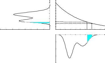
Fig. 3.8. Transformation of a probability density f(x) into g(u) via u(x). The shaded areas are equal.
3.4.1 Calculation of the Transformed Density
We consider a probability density f(x) and a monotone, i.e. uniquely invertible function u(x). We we are interested in the p.d.f. of u, g(u) (Fig. 3.8).
The relation P {x1 < x < x2} = P {u1 < u < u2} with u1 = u(x1), u2 = u(x2) has to hold, and therefore
Z x2
P {x1 < x < x2} = |
f(x′) dx′ |
|
Zxu1 2
= g(u′) du′ .
u1
This may be written in di erential form as
|g(u)du| = |f(x)dx| , |
(3.29) |
|||
|
|
dx |
|
|
|
|
|
|
|
g(u) = f(x) |
|
du |
. |
|
|
|
|
|
|
Taking the absolute value guarantees the positivity of the probability density. Integrating (3.29), we find numerical equality of the cumulative distribution functions, F (x) = G(u(x)).
If u(x) is not a monotone function, then, contrary to the above assumption, x(u) is not a unique function (Fig. 3.9) and we have to sum over the contributions of the
various branches of the inverse function: |
+ |
f(x) |
du |
|
+ · · · . |
(3.30) |
|||||
g(u) = |
f(x) |
du |
|
||||||||
|
|
|
dx |
|
|
|
|
dx |
|
|
|
|
|
|
|
|
|
|
|
|
|
|
|
|
|
|
|
|
|
|
|
|
|
|
|
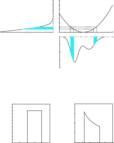
Example 22. Calculation of the p.d.f. for the volume of a sphere from the p.d.f. of the radius
40 3 Probability Distributions and their Properties
|
g(u) |
1.0 |
0.5 |
u |
|
|
|
6 |
|
u(x) |
|
|
|
|
|
4 |
|
|
|
2 |
|
|
|
00 |
5 |
10 |
x |
0. |
f(x) |
|
|
|
|
|
|
0.4 |
|
|
|
Fig. 3.9. Transformation of a p.d.f. f(x) into g(u) with u = x2. The sum of the shaded areas below f(x) is equal to the shaded area below g(u).
|
|
|
|
-3 |
|
|
|
|
|
|
4.0x10 |
|
|
0.50 |
|
|
|
g(V) |
|
|
f(r) |
|
|
|
|
|
|
|
|
|
|
|
|
|
|
|
|
|
-3 |
|
|
0.25 |
|
|
|
2.0x10 |
|
|
|
|
|
|
|
|
|
0.00 |
4 |
6 |
8 |
0.0 |
200 |
400 |
|
0 |
|||||
|
|
r |
|
|
|
V |
Fig. 3.10. Transformation of a uniform distribution of the radius into the distribution of the volume of a sphere.
Given a uniform distribution for the radius r |
|
|||
f(r) = |
1/(r |
2 − |
r ) if r < r < r |
|
0 |
1 else1 . |
2 |
||
we ask for the distribution g(V ) of the volume V (r). With
|
|
|
|
|
|
dr |
|
|
dV |
|
|
|
|
|
|
|
|
|
|
|
|
|
|
|
|
|
|
|
|
g(V ) = f(r) |
|
dV |
|
, |
dr |
= 4πr2 |
||||||||
we get |
|
|
|
|
|
|
|
|
|
|
|
|
|
|
g(V ) = |
|
1 |
|
1 |
|
= |
1 |
|
|
1 |
V −2/3. |
|||
|
− r1 4π r2 |
|
|
|
|
|||||||||
|
r2 |
|
|
V21/3 − V11/3 3 |
||||||||||
3.4 Transformation of Variables |
41 |
Example 23. Distribution of the quadratic deviation
For a normal distributed variate x with mean value x0 and variance s2 we ask for the distribution g(u), where
u = (x − x0)2/s2
is the normalized quadratic deviation. The expected value of u is unity, since the expected value of (x − µ)2 per definition equals σ2 for any distribution. The function x(u) has two branches. With
|
1 |
|
|
|
|
|
|
2 |
2 |
|||||
|
f(x) = |
|
√ |
|
|
|
e−(x−x0) |
/(2s ) |
||||||
|
|
|
|
s 2π |
|
|
||||||||
and |
|
|
|
|
dx |
|
|
s |
|
|
||||
|
|
|
|
|
|
|
|
|
||||||
|
|
|
|
|
|
|
= |
2√ |
|
|
|
|
||
|
|
|
|
|
du |
|
|
|||||||
|
|
|
|
|
u |
|
|
|
||||||
we find |
|
|
|
|
|
|
|
branch1 |
|
|
||||
g(u) = |
1 |
e−u/2 |
+ · · · branch2 . |
|||||||||||
2√ |
|
|||||||||||||
2πu |
||||||||||||||
The contributions from both branches are the same, thus
g(u) = √ 1 e−u/2 .
2πu
The function g(u) is the so-called χ2 - distribution for one degree of freedom.
(3.31)
(chi-square distribution)
Example 24. Distribution of kinetic energy in the one-dimensional ideal gas Be v the velocity of a particle in x direction with probability density
|
|
|
|
f(v) = r |
m |
2 |
|
|
e−mv |
/(2kT ). |
|
2πkT |
Its kinetic energy is E = v2/(2m), for which we want to know the distribution g(E). The function v(E) has again two branches. We get, in complete analogy to the example above,
|
|
|
dv |
= |
√ |
1 |
, |
|
|
|
|
|
|
|
|
|
|||
|
|
|
dE |
|
|
||||
g(E) = |
|
|
2mE |
|
|||||
1 |
|
e−E/kT branch1 |
+ · · · branch2. |
||||||
2√ |
|
||||||||
πkT E |
|||||||||
The contributions of both branches are the same, hence
g(E) = √ 1 e−E/kT . πkT E
3.4.2 Determination of the Transformation Relating two Distributions
In the computer simulation of stochastic processes we are frequently confronted with the problem that we have to transform the uniform distribution of a random number generator into a desired distribution, e.g. a normal or exponential distribution.

42 3 Probability Distributions and their Properties
More generally, we want to obtain for two given distributions f(x) and g(u) the transformation u(x) connecting them.
We have |
x |
u |
|
||
|
Z−∞ f(x′) dx′ = |
Z−∞ g(u′) du′ . |
Integrating, we get F (x) and G(u):
F (x) = G(u) ,
u(x) = G−1 (F (x)) .
G−1 is the inverse function of G. The problem can be solved analytically, only if f and g can be integrated analytically and if the inverse function of G can be derived.
Let us consider now the special case mentioned above, where the primary distribution f(x) is uniform, f(x) = 1 for 0 ≤ x ≤ 1. This implies F (x) = x and
G(u) = x, |
|
u = G−1(x) . |
(3.32) |
Example 25. Generation of an exponential distribution starting from a uniform distribution
Given are the p.d.f.s
f(x) =
g(u) =
1 for 0 < x < 1 0 else ,
λe−λu for 0 < u
0else .
The desired transformation u(x), as demonstrated above in the general case, is obtained by integration and inversion:
Z u Z x
g(u′) du′ = f(x′) dx′ ,
Z u0 Z0x
λe−λu′ du′ = f(x′) dx′ ,
0 0
1 − e−λu = x ,
u = − ln(1 − x)/λ .
We could have used, of course, also the relation (3.32) directly. Obviously in the last relation we could substitute 1 − x by x, since both quantities are uniformly distributed.
When we transform the uniformly distributed random numbers x delivered by our computer according to the last relation into the variable u, the latter will be exponentially distributed. This is the usual way to simulate the lifetime distribution of instable particles and other decay processes (see Chap. 5).
3.5 Multivariate Probability Densities
The results of the last sections are easily extended to multivariate distributions. We restrict ourself here to the case of continuous distributions8.
8An example of a multivariate discrete distribution will be presented in Sect. 3.6.2.

3.5 Multivariate Probability Densities |
43 |
3.5.1 Probability Density of two Variables
Definitions
As in the one-dimensional case we define an integral distribution function F (x, y), now taken to be the probability to find values of the variates x′, y′ smaller than x, respectively y
F (x, y) = P {(x′ < x) ∩ (y′ < y)} . |
(3.33) |
The following properties of this distribution function are satisfied:
F (∞, ∞) = 1,
F (−∞, y) = F (x, −∞) = 0 .
In addition, F has to be a monotone increasing function of both variables. We define a two-dimensional probability density, the so-called joined probability density, as the partial derivation of f with respect to the variables x, y:
f(x, y) = |
∂2F |
. |
|
∂x ∂y |
|||
|
|
From these definitions follows the normalization condition
Z ∞ Z ∞
f(x, y) dx dy = 1 .
−∞ −∞
The projections fx(x) respectively fy(y) of the joined probability density onto the coordinate axes are called marginal distributions :
Z ∞
fx(x) = f(x, y) dy ,
Z−∞∞
fy(y) = f(x, y) dx .
−∞
The marginal distributions are one-dimensional (univariate) probability densities.
The conditional probability densities for fixed values of the second variate and normalized with respect to the first one are denoted by fx(x|y) and fy(y|x) for given values of y or x, respectively. We have the following relations:
fx(x|y) =
=
fy(y|x) =
=
f(x, y)
R ∞ f(x, y) dx
−∞
f(x, y) , fy(y)
f(x, y)
R ∞ f(x, y) dy
−∞
f(x, y) .
Together, (3.34) and (3.35) express again Bayes’ theorem:
fx(x|y)fy(y) = fy(y|x)fx(x) = f(x, y) .
(3.34)
(3.35)
(3.36)

44 3 Probability Distributions and their Properties
Example 26. Superposition of two two-dimensional normal distributions9 The marginal distributions fx(x), fy(y) and the conditional p.d.f.
|
|
|
|
|
|
|
|
|
|
|
fy(y|x = 1) |
|
|
|
|
|
|
|
|
|
|
|
|
|
|
||||||||||
for the joined two-dimensional p.d.f. |
|
√3 |
− |
|
|
|
|
|
− |
|
|
−4 |
|
|
|
||||||||||||||||||||
|
|
2π |
|
|
|
|
− |
2 |
− 2 |
|
|
|
3 |
|
|
|
|
|
|
||||||||||||||||
f(x, y) = |
1 |
|
0.6 exp |
x2 |
|
y2 |
+ |
0.4 |
exp |
(x − 2)2 |
|
|
(y |
2.5)2 |
|
||||||||||||||||||||
|
|
|
|
|
|
|
|
|
|
|
|
|
|
|
|
|
|
|
|
|
|
||||||||||||||
are |
|
|
|
|
√2π |
|
|
− 2 |
|
|
|
|
√1.5 |
|
− |
|
|
|
|
|
|
|
|
||||||||||||
x |
|
|
|
|
|
|
|
|
|
|
|
3 |
|
|
|
|
|||||||||||||||||||
f |
(x) = |
1 |
|
0.6 exp |
|
|
|
x2 |
|
|
+ |
0.4 |
exp |
|
|
(x |
− |
2)2 |
|
|
, |
|
|
|
|||||||||||
|
|
|
|
− y2 |
|
|
|
|
|
|
|
|
|
|
|
|
|
|
|
|
|||||||||||||||
|
|
|
|
|
|
|
|
|
|
|
|
|
|
|
|
|
|
||||||||||||||||||
fy(y) = |
|
√2π 0.6 exp |
+ |
|
√2 exp − (y −42.5) |
, |
|
|
|
||||||||||||||||||||||||||
|
|
|
|
|
1 |
|
|
|
|
2 |
|
|
|
|
|
0.4 |
|
|
|
|
|
|
|
|
2 |
|
|
|
|
|
|
||||
f(y, x = 1) = 2π 0.6 exp − 2 − |
2 |
|
|
+ √3 exp |
− 3 − |
|
−4 |
|
|
, |
|||||||||||||||||||||||||
|
|
|
|
1 |
|
|
|
|
1 |
|
|
|
y2 |
|
|
0.4 |
|
|
|
|
1 |
|
|
(y |
2.5)2 |
|
|
|
|||||||
fy(y|x = 1) = 0.667 |
0.6 exp |
− 2 − y2 |
|
|
|
|
|
|
|
. |
|||||||||||||||||||||||||
+ √3 exp − 3 − (y −42.5) |
|||||||||||||||||||||||||||||||||||
|
|
|
|
|
|
|
|
|
|
1 |
|
|
2 |
0.4 |
|
|
|
|
|
1 |
|
|
|
|
|
2 |
|
||||||||
fy(y|1) and fR(y, 1) di er in the normalization factor, which results from the requirement fy(y|1) dy = 1.
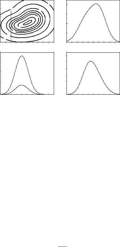
Graphical Presentation
Fig. 3.11 shows a similar superposition of two Gaussians together with its marginal distributions and one conditional distribution. The chosen form of the graphical representation as a contour plot for two-dimensional distributions is usually to be favored over three-dimensional surface plots.
3.5.2 Moments
Analogously to the one-dimensional case we define moments of two-dimensional distributions:
µx |
= E |
(x) , |
|
|
|
|
|
|
µy |
= E |
(y) , |
|
|
|
|
|
|
σx2 = E (x − µx)2 |
, |
|
|
|||||
σy2 = E |
(y − µy)2 |
, |
|
|
||||
|
|
[(x |
− |
µ |
)(y |
− |
µ |
)] , |
σxy = E |
x |
|
y |
|
||||
µlm = E(xlym), |
|
|
|
|
||||
µlm′ |
= E |
(x − µx)l(y − µy)m . |
||||||
Explicitly,
9The two-dimensional normal distribution will be discussed in Sect. 3.6.5.
3.5 Multivariate Probability Densities |
45 |
|
10 |
|
|
|
|
|
1E-3 |
|
|
1E-3 |
0.040 |
|
|
|
|
|
|
|
0.13 |
y |
5 |
|
|
|
|
|
|
|
|
|
0.17 |
|
|
|
0.070 |
|
|
0.010 |
|
|
|
1E-3 |
|
|
00 |
|
5 |
|
|
|
x |
|
0.3 |
|
|
|
|
|
f(y|x=2) |
|
0.2 |
|
|
|
0.1 |
|
f(y,x=2) |
|
0.00 |
|
5 |
|
|
|
y |
|
0.4 |
|
|
|
xf |
0.2 |
|
|
|
10 |
0.0 0 |
5 |
10 |
|
|
|
|
x |
|
|
0.6 |
|
|
|
|
0.4 |
|
|
|
yf |
|
|
|
|
|
0.2 |
|
|
|
10 |
0.0 |
0 |
5 |
10 |
|
|
|
y |
|
Fig. 3.11. Two-dimensional probability density. The lower left-hand plot shows the conditional p.d.f. of y for x = 2. The lower curve is the p.d.f. f(y, 2). It corresponds to the dashed line in the upper plot. The right-hand side displays the marginal distributions.
∞ |
∞ |
∞ |
µx = Z−∞ Z−∞ xf(x, y) dx dy = |
Z−∞ xfx(x) dx , |
|
∞ |
∞ |
∞ |
µy = Z−∞ Z−∞ yf(x, y) dx dy = |
Z−∞ yfy(y) dy , |
|
∞ |
∞ |
|
µlm = Z−∞ Z−∞ xlymf(x, y) dx dy , |
||
∞ |
∞ |
|
Z Z
µ′lm = (x − µx)l(y − µy)mf(x, y) dx dy .
−∞ −∞
Obviously, µ′x, µ′y (= µ′10, µ′01) are zero.
Correlations, Covariance, Independence
The mixed moment σxy is called covariance of x and y, and sometimes also denoted as cov(x, y). If σxy is di erent from zero, the variables x and y are said to be correlated. The mean value of y depends on the value chosen for x and vice versa. Thus, for instance, the weight of a man is positively correlated with its height.
The degree of correlation is quantified by the dimensionless quantity
ρxy = σxy ,
σxσy
46 3 Probability Distributions and their Properties
y |
y |
y |
y |
y |
x |
|
x |
|
x |
|
x |
|
x |
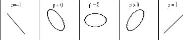
Fig. 3.12. Curves f(x, y) = const. with di erent correlation coe cients.
the correlation coe cient. Schwarz’ inequality insures |ρxy| ≤ 1.
Figure 3.12 shows lines of constant probability for various kinds of correlated distributions. In the extreme case |ρ| = 1 the variates are linearly related.
If the correlation coe cient is zero, this does not necessarily mean statistical independence of the variates. The dependence may be more subtle, as we will see shortly. As defined in Chap. 2, two random variables x, y are called independent or orthogonal, if the probability to observe one of the two variates x, y is independent from the value of the other one, i.e. the conditional distributions are equal to the marginal distributions, fx(x|y) = fx(x), fy(y|x) = fy(y). Independence is realized only if the joined distribution f(x, y) factorizes into its marginal distributions (see Chap. 2):
f(x, y) = fx(x)fy (y) .
Clearly, correlated variates cannot be independent.
Example 27. Correlated variates
A measurement uncertainty of a point in the xy-plane follows independent normal distributions in the polar coordinates r, ϕ (the errors are assumed small enough to neglect the regions r < 0 and |ϕ| > π ). A line of constant probability in the xy-plane would look similar to the second graph of Fig. 3.12. The cartesian coordinates are negatively correlated, although the original polar coordinates have been chosen as uncorrelated, in fact they are even independent.
Example 28. Dependent variates with correlation coe cient zero For the probability density
|
1 |
|
√ |
|
|
|
|
|
x2 |
+y2 |
|||
f(x, y) = |
|
|
|
e− |
|
|
|
|
|
||||
2πpx2 + y2 |
|
|
||||
|
|
|
|
|
||
we find σxy = 0. The curves f = const. are circles, but x and y are not independent, the conditional distribution fy(y|x) of y depends on x.
3.5.3 Transformation of Variables
The probability densities f(x, y) and g(u, v) are transformed via the transformation functions u(x, y), v(x, y), analogously to the univariate case