

vstatmp_engl
.pdf3.6 Some Important Distributions |
67 |
f(x) |
|
|
|
|
n=25 |
0.4 |
|
|
|
|
|
|
|
|
|
|
|
0.2 |
|
|
|
|
|
0.0 |
-4 |
-2 |
0 |
2 |
4 |
|
|||||
0.4 |
|
|
|
|
n=5 |
|
|
|
|
|
|
0.2 |
|
|
|
|
|
0.0 |
-4 |
-2 |
0 |
2 |
4 |
1.0 |
|
|
|
|
n=1 |
|
|
|
|
|
|
0.5 |
|
|
|
|
|
0.0 |
-4 |
-2 |
0x |
2 |
4 |
|
0.4 |
|
|
|
|
n=25 |
|
|
|
|
|
|
0.2 |
|
|
|
|
|
0.0 |
-4 |
-2 |
0 |
2 |
4 |
|
|||||
0.4 |
|
|
|
|
n=5 |
|
|
|
|
|
|
0.2 |
|
|
|
|
|
0.0 |
-4 |
-2 |
0 |
2 |
4 |
|
|||||
0.4 |
|
|
|
|
n=1 |
|
|
|
|
|
|
0.2 |
|
|
|
|
|
0.0 |
-4 |
-2 |
0 |
2 |
4 |
|
|||||
|
|
|
x |
|
|
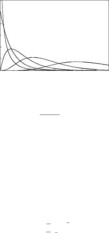
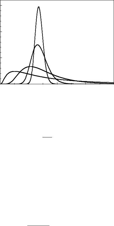
Fig. 3.18. Illustration of the central limit theorem. The uniformly distributed variates approach with increasing n
mean values of n exponential or the normal distribution.
68 3 Probability Distributions and their Properties
y |
s |
|
|
|
|
|
y |
|
s' |
s |
|
y |
|
|
|
x |
|
s' |
|
x' |
|
|
|
x |
y' |
|
|
|
|
|
|
x |
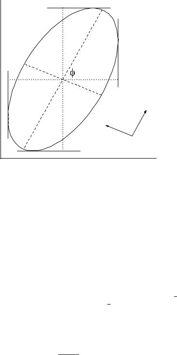
Fig. 3.19. Transformation of the error ellipse.
We skip the explicit calculation. Integrating (3.49) over y, (x), we obtain the marginal distributions of x, (y). They are again normal distributions with widths sx and sy. A characteristic feature of the normal distribution is that for a vanishing correlation ρ = 0 the two variables are independent, since in this case the p.d.f. N0(x, y) factorizes into normal distributions of x and y.
Curves of equal probability are obtained by equating the exponent to a constant.
The equations |
|
x2 |
|
|
|
y2 |
= const |
|
1 |
− 2ρ |
xy |
+ |
|||||
|
1 − ρ2 |
sx2 |
sxsy |
sy2 |
||||
describe concentric ellipses. For the special choice const = 1 we show the ellipse in Fig. 3.19. At this so-called error ellipse the value of the p.d.f. is just N0(0, 0)/√e, i.e. reduced with respect to the maximum by a factor 1/√e.
By a simple rotation we achieve uncorrelated variables x′ and y′:
x′ = x cos φ + y sin φ , y′ = −x sin φ + y cos φ ,
tan 2φ = 2ρsxsy . s2x − s2y
The half-axes, i.e. the variances s′x2 and s′y2 of the uncorrelated variables x′ and y′ are
3.6 Some Important Distributions |
69 |
s′2 |
= |
sx2 + sy2 |
+ |
sx2 − sy2 |
, |
|
|
||||
x |
2 |
|
2 cos 2φ |
|
|
|
|
|
|||
s′2 |
= |
sx2 + sy2 |
− |
sx2 − sy2 |
. |
|
2 cos 2φ |
||||
y |
2 |
|
|||
In the new variables, the normal distribution has then the simple form
N0′ (x′, y′) = 2πsx′ |
sy′ |
exp |
− 2 |
sx′ 2 |
+ sy′ 2 |
|
= f(x′)g(y′) . |
||
1 |
|
|
1 |
|
x′2 |
|
y′2 |
|
|
The two-dimensional normal distribution with its maximum at (x0, y0) is obtained from (3.49) with the substitution x → x − x0, y → y − y0.
We now generalize the normal distribution to n dimensions. We skip again the simple algebra and present directly the result. The variables are written in vector form x and with the symmetric and positive definite covariance matrix C, the p.d.f. is given by
N(x) = |
|
1 |
|
− |
1 |
(x − x0)T C−1(x − x0) . |
|
(2π)n det(C) exp |
2 |
||||
|
p |
|
|
|
|
|
Frequently we need the inverse of the covariance matrix
V = C−1
which is called weight matrix. Small variances Cii of components xi lead to large weights Vii. The normal distribution in n dimensions has then the form
N(x) = |
|
1 |
|
− |
1 |
(x − x0)T V(x − x0) . |
|
(2π)n det(C) exp |
2 |
||||
|
p |
|
|
|
|
|
In the two-dimensional case the matrices C and V are
C = |
sx2 |
ρsxsy |
|
, |
|
|
|
||||||
|
|
sy2 |
|
|
|
||||||||
|
ρsxsy |
|
ρ |
! |
|||||||||
|
|
|
1 |
|
1 |
|
|
|
− |
||||
V |
= |
|
|
|
sx2 |
|
|
|
sxsy |
||||
|
|
− ρ2 |
− |
ρ |
|
|
1 |
|
|||||
|
1 |
sxsy |
|
|
sy2 |
|
|||||||
with the determinant det(C) = s2xs2y(1 − ρ2) = 1/ det(V).
3.6.6 The Exponential Distribution
Also the exponential distribution appears in many physical phenomena. Besides life time distributions (decay of instable particles, nuclei or excited states), it describes the distributions of intervals between Poisson distributed events like time intervals between decays or gap lengths in track chambers, and of the penetration depth of particles in absorbing materials.
The main characteristics of processes described by the exponential distribution is lack of memory, i.e. processes which are not influenced by their history. For instance, the decay probability of an instable particle is independent of its age, or the scattering probability for a gas molecule at the time t is independent of t and of the time that

70 3 Probability Distributions and their Properties
has passed since the last scattering event. The probability density for the decay of a particle at the time t1 + t2 must be equal to the probability density f(t2) multiplied with the probability 1 − F (t1) to survive until t1:
f(t1 + t2) = (1 − F (t1)) f(t2) .
Since f(t1 + t2) must be symmetric under exchanges of t1 and t2, the first factor has to be proportional to f(t1),
1 − F (t1) = cf(t1) , |
(3.50) |
f(t1 + t2) = cf(t1)f(t2) |
(3.51) |
with constant c. The property (3.51) is found only for the exponential function: f(t) = aebt. If we require that the probability density is normalized, we get
f(t) = λe−λt .
This result could also have been derived by di erentiating (3.50) and solving the corresponding di erential equation f = −c df/dt.
The characteristic function
λ
φ(t) = λ − it
and the moments
µn = n! λ−n
have already been derived in Example 21 in Sect. 3.3.3.
3.6.7 The χ2 Distribution
The chi-square distribution (χ2 distribution) plays an important role in the comparison of measurements with theoretical distributions (see Chap. 10). The corresponding tests allow us to discover systematic measurement errors and to check the validity of theoretical models. The variable χ2 which we will define below, is certainly the quantity which is most frequently used to quantify the quality of the agreement of experimental data with the theory.
The variate χ2 is defined as the sum
Xf x2
χ2 = σi2 ,
i=1 i
where xi are independent, normally distributed variates with zero mean and variance
σi2.
We have already come across the simplest case with f = 1 in Sect. 3.4.1: The transformation of a normally distributed variate x with expected value zero to u = x2/s2, where s2 is the variance, yields
g1 |
(u) = |
√ |
1 |
e−u/2 |
(f = 1) . |
|
|
|
2πu |
|
|
(We have replaced the variable χ2 by u = χ2 |
to simplify the writing.) Mean value |
||||
and variance of this distribution are E(u) = 1 and var(u) = 2.
3.6 Some Important Distributions |
71 |
0.6 |
|
|
|
|
|
|
f=1 |
|
|
|
|
0.4 |
|
|
|
|
|
|
f=2 |
|
|
|
|
0.2 |
f=4 |
|
|
|
|
|
f=8 |
|
|
|
|
|
|
|
f=16 |
|
|
|
|
|
|
|
|
0.00 |
5 |
10 |
c 2 |
15 |
20 |
|
|
|
|
|
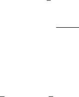
Fig. 3.20. χ2distribution for di erent degrees of freedom.
When we now add f independent summands we obtain
|
1 |
|
gf (u) = |
Γ (f/2)2f/2 uf/2−1e−u/2 . |
(3.52) |
The only parameter of the χ2 distribution is the number of degrees of freedom f, the meaning of which will become clear later. We will prove (3.52) when we discuss the gamma distribution, which includes the χ2 distribution as a special case. Fig. 3.20 shows the χ2 distribution for some values of f. The value f = 2 corresponds to an exponential distribution. As follows from the central limit theorem, for large values of f the χ2 distribution approaches a normal distribution.
By di erentiation of the p.d.f. we find for f > 2 the maximum at the mode
umod = f − 2. The expected value of the variate u is equal to f and its variance is 2f. These relations follow immediately from the definition of u.
umod = f − 2 for f > 2 , E(u) = f ,
var(u) = 2f .
Distribution of the Sample Width
We define the width v of a sample of N elements xi as follows (see 3.2.3):
v2 = N1 XN x2i − x2
i=1
= x2 − x2 .

72 3 Probability Distributions and their Properties
If the variates xi of the sample are distributed normally with mean x0 and variance σ2, then Nv2/σ2 follows a χ2 distribution with f = N − 1 degrees of freedom. We omit the formal proof; the result is plausible, however, from the expected value derived in Sect. 3.2.3:
|
Nv2 |
|
|
|
N |
|
|
v2 |
|
= |
N − 1 |
σ2 , |
|
|
|
|
= N − 1 . |
|||
σ2 |
||||||
Degrees of Freedom and Constraints
In Sect. 7.2 we will discuss the method of least squares for parameter estimation. To adjust a curve to measured points xi with Gaussian errors σi we minimize the quantity
|
|
(t) |
(λ1, . . . , λZ ) |
|
2 |
|
|
|
|
|
|
||
|
N |
x x |
|
|
|
|
|
i − i |
|
|
|
|
|
χ2 = |
Xi |
|
|
, |
||
|
|
σ2 |
|
|
||
|
=1 |
|
i |
|
|
|
|
|
|
|
|
|
where x(it) are the ordinates of the curve depending on the Z free parameters λk. Large values of χ2 signal a bad agreement between measured values and the fitted curve. If the predictions x(it) depend linearly on the parameters, the sum χ2 obeys a χ2 distribution with f = N − Z degrees of freedom. The reduction of f accounts for the fact that the expected value of χ2 is reduced when we allow for free parameters. Indeed, for Z = N we could adjust the parameters such that χ2 would vanish.
Generally, in statistics the term degrees of freedom13 f denotes the number of independent predictions. For N = Z we have no prediction for the observations xi. For Z = 0 we predict all N observations, f = N. When we fit a straight line through 3 points with given abscissa and observed ordinate, we have N = 3 and Z = 2 because the line contains 2 parameters. The corresponding χ2 distribution has 1 degree of freedom. The quantity Z is called the number of constraints, a somewhat misleading term. In the case of the sample width discussed above, one quantity, the mean, is adjusted. Consequently, we have Z = 1 and the sample width follows a χ2 distribution of f = N − 1 degrees of freedom.
3.6.8 The Gamma Distribution
The distributions considered in the last two sections, the exponentialand the chisquare distribution, are special cases of the gamma distribution
G(x|ν, λ) = |
λν |
Γ (ν) xν−1e−λx , x > 0 . |
The parameter λ > 0 is a scale parameter, while the parameter ν > 0 determines the shape of the distribution. With ν = 1 we obtain the exponential distribution. The parameter ν is not restricted to natural numbers. With the special choice ν = f/2 and λ = 1/2 we get the χ2-distribution with f degrees of freedom (see Sect. 3.6.7).
13Often the notation number of degrees of freedom, abbreviated by n.d.f. or NDF is used in the literature.
3.6 Some Important Distributions |
73 |
The gamma distribution is used typically for the description of random variables that are restricted to positive values, as in the two cases just mentioned. The characteristic function is very simple:
φ(t) = 1 − |
t |
|
−ν |
|
i |
. |
(3.53) |
||
λ |
As usual, we obtain expected value, variance, moments about the origin, skewness and excess by di erentiating φ(t):
|
ν |
, var(x) = |
ν |
|
Γ (i + ν) |
2 |
|
6 |
|
||
hxi = |
|
|
, µi = |
|
, γ1 = √ |
|
, γ2 = |
|
. |
||
λ |
λ2 |
λi Γ (ν) |
ν |
||||||||
ν |
|||||||||||
The maximum of the distribution is at xmod = (ν − 1)/λ, (ν > 1).
The gamma distribution has the property of stability in the following sense: The sum of variates following gamma distributions with the same scaling parameter λ, but di erent shape parameters νi is again gamma distributed, with the shape parameter
ν, X
ν = νi .
This result is obtained by multiplying the characteristic functions (3.53). It proves also the corresponding result (3.52) for the χ2-distribution.
Example 42. Distribution of the mean value of decay times
P
Let us consider the sample mean x = xi/N, of exponentially distributed variates xi. The characteristic function is (see 3.3.3)
1
φx(t) = 1 − it/λ .
Forming the N-fold product, and using the scaling rule for Fourier transforms (3.19), φx/N (t) = φx(t/N), we arrive at the characteristic function of a gamma distribution with scaling parameter Nλ and shape parameter N:
|
|
(t) = 1 − |
it |
|
−N |
(3.54) |
φ |
|
|
. |
|||
x |
Nλ |
Thus the p.d.f. f(x) is equal to G(x|N, Nλ). Considering the limit for large N, we convince ourself of the validity of the law of large numbers and the central limit theorem. From (3.54) we derive
ln φ |
|
(t) = −N ln 1 − |
|
|
|
it |
|
|
|
|
|
|
||||||
|
|
|
|
|
|
|
|
|
||||||||||
x |
Nλ |
|
|
|
|
|
||||||||||||
|
|
|
|
|
|
it |
|
|
|
1 |
|
|
it |
2 |
|
|||
|
|
= −N " |
|
|
|
− |
|
|
+ O(N−3)# |
, |
||||||||
|
|
− Nλ |
|
2 |
− Nλ |
|||||||||||||
|
|
|
|
|
|
|
|
|
|
|
|
|
|
|
|
|||
|
|
|
1 |
1 |
|
1 |
|
|
|
|
N−2 . |
|
||||||
φ |
|
(t) = exp i |
|
t − |
|
|
|
t2 + O |
|
|||||||||
x |
λ |
2 |
Nλ2 |
|
||||||||||||||
When N is large, the term of order N−2 can be neglected and with the two remaining terms in the exponent we get the characteristic function of a normal distribution with mean µ = 1/λ = hxi and variance σ2 = 1/(Nλ2) =
74 3 Probability Distributions and their Properties
|
2.0 |
|
|
|
1.5 |
|
|
f(x) |
1.0 |
|
|
|
0.5 |
|
|
|
0.0 0 |
1 |
2 |
|
|
x |
|
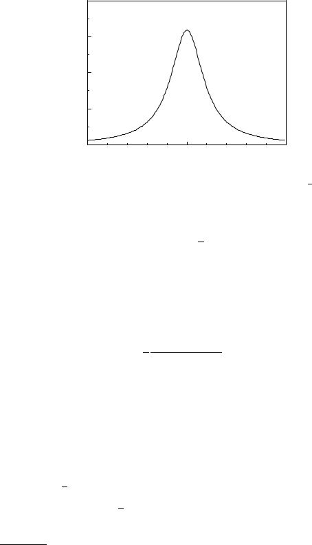
Fig. 3.21. Lorentz distribution with mean equal to 1 and halfwidth /2 = √2.
var(x)/N, (see 3.3.3), in agreement with the central limit theorem. If N approaches infinity, only the first term remains and we obtain the characteristic function of a delta distribution δ(1/λ − x). This result is predicted by the law of large numbers (see Appendix 13.1). This law states that, under certain conditions, with increasing sample size, the di erence between the sample mean and the population mean approaches zero.
3.6.9 The Lorentz and the Cauchy Distributions
The Lorentz distribution (Fig. 3.21)
1Γ/2
f(x) = π (x − a)2 + (Γ/2)2
is symmetric with respect to x = a. Although it is bell-shaped like a Gaussian, it has, because of its long tails, no finite variance. This means that we cannot infer the location parameter a of the distribution14 from the sample mean, even for arbitrary large samples. The Lorentz distribution describes resonance e ects, where Γ represents the width of the resonance. In particle or nuclear physics, mass distributions of short-lived particles follow this p.d.f. which then is called Breit–Wigner distribution.
The Cauchy distribution corresponds to the special choice of the scale parameter Γ = 2. 15 For the location parameter a = 0 it has the characteristic function φ(t) = exp(−|t|), which obviously has no derivatives at t = 0, an other consequence of the nonexistence of moments. The characteristic function for the sample mean of N measurements, x = PN1 xi/N, is found with the help of (3.19), (3.25) as
φx(t) = (φ(t/N))N = φ(t) .
The sample mean has the same distribution as the original population. It is therefore, as already stated above, not suited for the estimation of the location parameter.
14The first moment exists only as a Cauchy principal value and equals a.
15In the literature also the more general definition with two parameters is met.

3.6 Some Important Distributions |
75 |
3.6.10 The Log-normal Distribution
The distribution of a variable x > 0 whose logarithm u is normally distributed
g(u) = √1 e−(u−u0)2/2s2
2πs
with mean u0 and variance s2 follows the log-normal distribution, see Fig. 3.22:
1 |
2 |
2 |
||
f(x) = |
√ |
|
e−(ln x−u0) |
/2s . |
|
xs |
2π |
|
|
This is, like the normal distribution, a two-parameter distribution where the parameters u0, s2, however, are not identical with the mean µ and variance σ2, but the latter are given by
µ = eu0+s2/2, |
|
σ2 = (es2 − 1)e2u0+s2 . |
(3.55) |
Note that the distribution is declared only for positive x, while u0 can also be negative.
The characteristic function cannot be written in closed form, but only as a power expansion. This means, the moments of order k about the origin are
µk = e |
ku0+ |
21 k2s2 |
. |
|
|
|
|
||
|
|
|
|
|
|
|
|||
Other characteristic parameters are |
|
|
|
|
|
|
|
|
|
median : x0.5 |
= eu0 , |
|
|
|
|
|
|
|
|
mode : xmod |
= eu0−s2 |
, |
|
|
|
|
|
|
|
skewness : γ1 |
= (es2 + 2) |
|
, |
|
|
||||
es2 − 1 |
|
|
|||||||
kurtosis : γ2 |
|
2 |
3s2 |
+ 3e |
2s2 |
− 6 . |
(3.56) |
||
= e4s + 2ep |
|
|
|||||||
The distribution of a variate x = Yxi |
which is the product of many variates |
||||||||
xi, each of which is positive and has a small variance, σi2 compared to its mean squared µ2, σi2 µ2i , can be approximated by a log-normal distribution. This is a consequence of the central limit theorem (see 3.6.5). Writing
N |
|
Xi |
ln xi |
ln x = |
|
=1 |
|
we realize that ln x is normally distributed in the limit N → ∞ if the summands fulfil the conditions required by the central limit theorem. Accordingly, x will be distributed by the log-normal distribution.
3.6.11 Student’s t Distribution
This distribution, introduced by W. S. Gosset (pseudonym “Student”) is frequently used to test the compatibility of a sample with a normal distribution with given mean
76 3 Probability Distributions and their Properties
1.5 |
|
|
|
|
|
|
f(x) |
|
|
s=0.1 |
|
|
|
|
|
|
|
|
|
|
1.0 |
|
|
|
|
|
|
0.5 |
|
|
|
|
|
|
|
s=1 |
s=0.5 |
s=0.2 |
|
|
|
|
|
|
|
|
|
|
0.00 |
|
2 |
4 |
x |
6 |
8 |
|
|
|
|
|
|
Fig. 3.22. Log-normal distribution with u0 = 1 and di erent values of s.
but unknown variance. It describes the distribution of the so-called “studentized” variate t, defined as
t = |
|
− µ |
. |
|
x |
(3.57) |
|||
|
||||
|
|
s |
|
|
The numerator is the di erence between a sample mean and the mean of the Gaussian from which the sample of size N is drawn. It follows a normal distribution centered at zero. The denominator s is an estimate of the standard deviation of the numerator derived from the sample. It is defined by (3.15).
|
|
− |
N |
|||
|
1 |
Xi |
||||
s2 = |
|
|
(xi − |
x |
)2 . |
|
N(N 1) |
||||||
|
|
|
|
=1 |
|
|
The sum on the right-hand side, after division by the variance σ2 of the Gaussian,
follows a χ2 distribution with f = N − 1 degrees of freedom, see (3.52). Dividing
√
also the numerator of (3.57) by its standard deviation σ/ N, it follows a normal distribution of variance unity. Thus the variable t of the t distribution is the quotient of a normal variate and the square root of a χ2 variate.
The analytical form of the p.d.f. can be found by the standard method used in Sect. 3.5.4. The result is
|
Γ ((f + 1)/2) |
2 |
|
− f+12 |
|||||
h(t|f) = |
Γ (f/2)√ |
|
|
|
1 + |
t |
|
. |
|
f |
|||||||||
πf |
|
||||||||