vstatmp_engl

with tiny values for δπ and δε.

This direct inclusion of the constraint through a penalty term in the fit is technically very simple and e cient.

As demonstrated in example 88 the term su ciently small means that the uncertainty δhk of a constraint k as derived from the fitted values of the parameters and their errors is large compared to δk:

The quantities δθi in (6.24) are not known precisely before the fit is performed but can be estimated su ciently well beforehand. The precise choice of the constraint precision δk is not at all critical, variations by many orders of magnitude make no di erence but a too small values of δk could lead to numerical problems.

6.6.4 The Method of Lagrange Multipliers

This time we choose the likelihood presentation of the problem. The likelihood function is extended to

We have appended an expressions that in the end should be equal to zero, the constraint functions multiplied by the so-called Lagrange multipliers. The MLE as obtained by setting ∂ ln L/∂θj = 0 yields parameters that depend on the Lagrange multipliers α. We can now use the free parameters αk to fulfil the constraints, or in other words, we use the constraints to eliminate the Lagrange multiplier dependence of the MLE.

Example 93. Example 88 continued

Our full likelihood function is now

168 6 Parameter Inference I

Of course, the general situation is much more complicated than that of our trivial example. An analytic solution will hardly be possible. Instead we can set the derivative of the log-likelihood not only with respect to the parameters θ but also with respect to the multipliers αk equal to zero, ∂ ln L/∂αk = 0, which automatically implies, see (6.25), that the constraints are satisfied. Unfortunately, the zero of the derivative corresponds to a saddle point and cannot be found by a maximum searching routine. More subtle numerical methods have to be applied.

Most methods avoid this complication and limit themselves to linear regression models which require a linear dependence of the observations on the parameters and linear constraint relations. Non-linear problems are then solved iteratively. The solution then is obtained by a simple matrix calculus.

Linear regression will be sketched in Sect. 7.2.3 and the inclusion of constraints in Appendix 13.10.

6.6.5 Conclusion

By far the simplest method is the one where the constraint is directly included and approximated by a narrow Gaussion. With conventional minimizing programs the full error matrix is produced automatically.

The approach using a reduced parameter set is especially interesting when we are primarily interested in the parameters of the reduced set. Due to the reduced dimension of the parameter space, it is faster than the other methods. The determination of the errors of the original parameters through error propagation is sometimes tedious.

It is recommended to either eliminate redundant parameters or to use the simple method where we represent constraints by narrow Gaussians. The application of Lagrange multipliers is unnecessarily complicated and the linear approximation requires additional assumptions and iterations.

6.7 Reduction of the Number of Variates

6.7.1 The Problem

A statistical analysis of an univariate sample is obviously much simpler than that of a multidimensional one. This is not only true for the qualitative comparison of a sample with a parameter dependent p.d.f. but also for the quantitative parameter inference. Especially when the p.d.f. is distorted by the measurement process and a Monte Carlo simulation is required, the direct ML method cannot be applied as we have seen above. The parameter inference then happens by comparing histograms with the problem that in multidimensional spaces the number of entries can be quite small in some bins. Therefore, we have an interest to reduce the dimensionality of the variable space by appropriate transformations, of course, if possible, without loss of information. However, it is not always easy to find out which variable or which variable combination is especially important for the parameter estimation.

Fig. 6.13. Simulated p.d.f.s of the reduced variable u for the values ±1 of the parameter.

Example 94. Reduction of the variate space We consider the p.d.f.

f(x, y, z|θ) = π1 h(x2 + y2 + z2)1/2 + (x + y3)θi , x2 + y2 + z2 ≤ 1 , (6.27)

which depends on three variates and one parameter. For a given sample of observations in the three dimensional cartesian space we want to determine the parameter θ. The substitutions

v = (x2 + y2 + z2)1/2 , 0 ≤ v ≤ 1 ,

z = z

lead to the new p.d.f. g′(u, v, z)

which after integrating out v and z yields the p.d.f. g(u|θ):

Z

g(u|θ) = dz dv g′(u, v, z|θ) .

This operation is not possible analytically but we do not need to compute g explicitly. We are able to determine the MLE and its error from the simple log-likelihood function of θ

X

ln L(θ) = ln(1 + uiθ) .

i

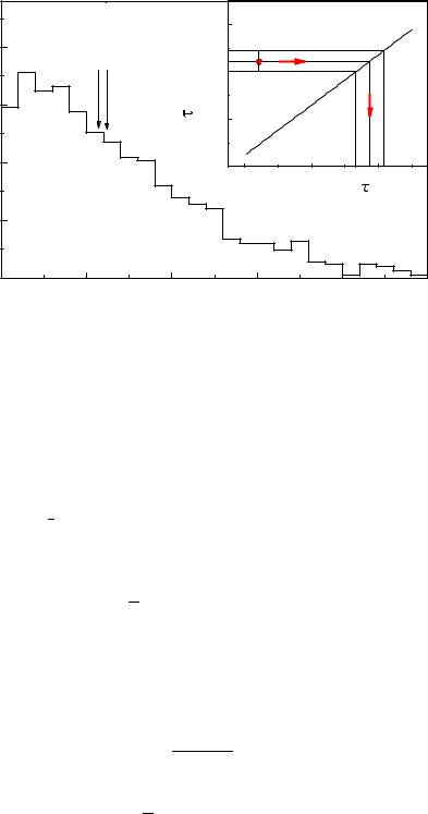
Fig. 6.14. Observed lifetime distribution. The insert indicates the transformation of the observed lifetime to the corrected one.

obtain when we insert the data into the undistorted p.d.f.. In both cases we find the relation between the experimental statistic and the estimate of the parameter by a Monte Carlo simulation. The method should become clear in the following example.

Example 95. Approximated likelihood estimator: Lifetime fit from a distorted distribution

The sample mean t of a sample of N undistorted exponentially distributed lifetimes ti is a su cient estimator: It contains the full information related to the parameter τ, the mean lifetime (see Sect. 7.1.1). In case the distribution is distorted by resolution and acceptance e ects (Fig. 6.14), the mean value

X

t′ = t′i/N

of the distorted sample t′i will usually still contain almost the full information relative to the mean life τ. The relation τ(t′) between τ and its approximation t′ (see insert of Fig. 6.14) is generated by a Monte Carlo simulation. The uncertainty δτ is obtained by error propagation from the uncertainty δt′ of t′,

using the Monte Carlo relation τ(t′).

This approach has several advantages:

•We do not need to histogram the observations.

•Problems due to small event numbers for bins in a multivariate space are avoided.

•It is robust, simple and requires little computing time.

For these reasons the method is especially suited for online applications, provided that we find an e cient estimator.

If the distortions are not too large, we can use the likelihood estimator extracted from the observed sample {x′1, . . . , x′N } and the undistorted distribution f(x|λ):

Y

L(λ) = f(x′i|λ) ,

dL

d |ˆ = 0 . (6.29)

λ λ′

This means concretely that we perform the usual likelihood analysis where we ignore

the distortion. We obtain ˆ′. Then we correct the bias by a Monte Carlo simulation

λ

which provides the relation ˆ ˆ′ .

λ(λ )

It may happen in rare cases where the experimental resolution is very bad that f(x|λ) is undefined for some extremely distorted observations. This problem can be

cured by scaling ˆ′ or by eliminating particular observations.

λ

Acceptance losses α(x) alone without resolution e ects do not necessarily entail a reduction in the precision of our approach. For example, as has been shown in Sect. 6.5.2, cutting an exponential distribution at some maximum value of the variate, the mean value of the observations is still a su cient statistic. But there are cases where sizable acceptance losses have the consequence that our method deteriorates. In these cases we have to take the losses into account. We only sketch a suitable method. The acceptance corrected p.d.f. f′(x|λ) for the variate x is

where the denominator is the global acceptance and provides the correct normalization. We abbreviate it by A(λ). The log-likelihood of N observations is

XX

ln L(λ) = ln α(xi) + ln f(xi|λ) − NA(λ) .

The first term can be omitted. The acceptance A(λ) can be determined by a Monte Carlo simulation. Again a rough estimation is su cient, at most it reduces the precision but does not introduce a bias, since all approximations are automatically corrected with the transformation λ(λ′).

Frequently, the relation (6.29) can only be solved numerically, i.e. we find the maximum of the likelihood function in the usual manner. We are also allowed to approximate this relation such that an analytic solution is possible. The resulting error is compensated in the simulation.

Example 96. Approximated likelihood estimator: linear and quadratic distributions

A sample of events xi is distributed linearly inside the interval [−1, 1], i.e. the p.d.f. is f(x|b) = 0.5 + bx. The slope b , |b| < 1/2, is to be fitted. It is located in the vicinity of b0. We expand the likelihood function

where we have set f0i = f(xi|b0).

If we allow also for a quadratic term

f(x|a, b) = a + bx + (1.5 − 3a)x2 ,

we write, in obvious notation,

f(x|a, b) = f0 + α(1 − 3x2) + βx

and get, after deriving ln L with respect to α and β and linearizing, two linear

with the abbreviations Ai = (1 − 3x2i )/f0i, Bi = xi/f0i.

From the observed data using (6.31) we get ˆ′ ′ , ′ ′ , and the simulation

β (x ) αˆ (x )

provides the parameter estimates ˆ ˆ′ ′ and their uncertainties. b(β ), aˆ(αˆ )

The calculation is much faster than a numerical minimum search and almost as

precise. If ˆ are large we have to iterate.

α,ˆ β

6.9 Nuisance Parameters

Frequently a p.d.f. f(x|θ, ν) contains several parameters from which only some, namely θ, are of interest, whereas the other parameters ν are unwanted, but influence the estimate of the former. Those are called nuisance parameters. A typical example is the following.

Example 97. Nuisance parameter: decay distribution with background

We want to infer the decay rate γ of a certain particle from the decay times ti of a sample of M events. Unfortunately, the sample contains an unknown amount of background. The decay rate γb of the background particles be known. The nuisance parameter is the number of background events N. For

number of background events

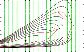
Fig. 6.15. Log-likelihood contour as a function of decay rate and number of background events. For better visualization the discrete values of the event numbers are connected.

Let us resume the problem discussed in the introduction. We now assume that we have prior information on the amount of background: The background expectation had been determined in an independent experiment to be 10 with su cient precision to neglect its uncertainty. The actual number of background events follows a Poisson distribution. The likelihood function is

Since our nuisance parameter is discrete we have replaced the integration in (6.32) by a sum.

6.9.2 Factorizing the Likelihood Function

Very easy is the elimination of the nuisance parameter if the p.d.f. is of the form

i.e. only the first term fθ depends on θ. Then we can write the likelihood as a product

L(θ, ν) = Lθ(θ)Lν (ν)

Lθ = fθ(xi|θ) ,

independent of the nuisance parameter ν.

Example 99. Elimination of a nuisance parameter by factorization of a twodimensional normal distribution