vstatmp_engl

XN

ln L(τ) = −ni(ln τ + τˆi/τ)

i=1

= −n ln τ − X niτˆi

τ

with the maximum at P niτˆi

τˆ =

n

and its error

τˆ

δ = √n .

The individual measurements are weighted by their event numbers, instead of weights proportional to 1/δi2. As the errors are correlated with the measurements, the standard weighted mean (4.7) with weights proportional to 1/δi2 would be biased. In our specific example the correlation of the errors and the parameter values is known and we could use weights proportional to

(τi/δi)2.

Example 117. Averaging ratios of Poisson distributed numbers

In absorption measurements and many other situations we are interested in a parameter which is the ratio of two numbers which follow the Poisson distri-

bution. Averaging naively these ratios ˆ using the weighted mean

θi = mi/ni

(4.7) can lead to strongly biased results. Instead we add the log-likelihood functions which we have derived in Sect. 6.9.3

In the standard situation where we do not know the full likelihood function but only the MLE and the error limits we have to be content with an approximate procedure. If the likelihood functions which have been used to extract the error limits are parabolic, then the standard weighted mean (4.7) is exactly equal to the result which we obtain when we add the log-likelihood functions and extract then the estimate and the error.

Proof: A sum of terms of the form (8.1) can be written in the following way:

Since the right hand side is the most general form of a polynomial of second order, a comparison of the coe cients of θ2 and θ yields

X

V θ = Viθi ,

where c is a number which has to be large compared to the absolute change of θ within the ln L = 1/2 region. We get µlow and θlow = θ(µlow) and maximizing

θ(µ) − c [ln L(µb) − ln L(µ) − 1/2]2

we get θup.

If the likelihood functions are not known, the only practical way is to resort to a Bayesian treatment, i.e. to make assumptions about the p.d.f.s of the input parameters. In many cases part of the input parameters have systematic uncertainties. Then, anyway, the p.d.f.s of those parameters have to be constructed. Once we have established the complete p.d.f. f(µ), we can also determine the distribution of θ. The analytic parameter transformation and reduction described in Chap. 3 will fail in most cases and we will adopt the simple Monte Carlo solution where we generate a sample of events distributed according to f(µ) and where θ(µ) provides the θ distribution in form of a histogram and the uncertainty of this parameter. To remain consistent with our previously adopted definitions we would then interpret this p.d.f.

of as a likelihood function and derive from it the MLE ˆ and and the likelihood

θ θ

ratio error limits.

We will not discuss the general scheme in more detail but add a few remarks related to special situations and discuss two simple examples.

Sum of Many Measurements

If the output parameter θ = P ξi is a sum of “many” input quantities ξi with variances σi2 of similar size and their mean values and variances are known, then due to the central limit theorem we have

ˆ h i h i

θ = θ = Σ ξi , δθ2 = σθ2 ≈ Σσi2

independent of the shape of the distributions of the input parameters and the error of θ is normally distributed. This situation occurs in experiments where many systematic uncertainties of similar magnitude enter in a measurement.

Product of Many Measurements

Y

If the output parameter θ = ξi is a product of “many” positive input quantities ξi with relative uncertainties σi/ξi of similar size then due to the central limit theorem

hln θi = Σhln ξii , q

σln θ ≈ Σσln2 ξi

independent of the shape of the distributions of the input parameters and the error of ln θ is normally distributed which means that θ follows a log-normal distribution (see Sect. 3.6.10). Such a situation may be realized if several multiplicative e ciencies

is that the number of equivalent events is large enough to use symmetric errors. If this number is low we derive the limits from the Poisson distribution of the equivalent number of events which then will be asymmetric.

Example 119. Sum of weighted Poisson numbers

Particles are detected in three detectors with e ciencies ε1 = 0.7, ε2 = 0.5, ε3 = 0.9. The observed event counts are n1 = 10, n2 = 12, n3 = 8.

A background contribution is estimated in a separate counting experiment as b = 9 with a reduction factor of r = 2. The estimate nˆ for total number of particles which traverse the detectors is nˆ = P ni/εi − b/r = 43. From linear error propagation we obtain the uncertainty δn = 9. A more precise calculation based on the Poisson distribution of the equivalent number of events would yield asymmetric errors, nˆ = 43 .

Averaging Correlated Measurements

The following example is a warning that naive linear error propagation may lead to false results.

Example 120. Average of correlated cross section measurements, Peelle’s pertinent puzzle

The results of a cross section measurements is ξ1 with uncertainties due to the event count, δ10, and to the beam flux. The latter leads to an error δf ξ which is proportional to the cross section ξ. The two contributions are independent and thus the estimated error squared in the Gaussian approximation is δ12 = δ102 + δf2 ξ12. A second measurement ξ2 with di erent statistics but the same

uncertainty on the flux has an uncertainty δ22 = δ202 + δf2 ξ22. Combining the two measurements we have to take into account the correlation of the errors. In the literature [45] the following covariance matrix is discussed:

It can lead to the strange result that the least square estimate b of the two

ξ

section

cross sections is located outside the range defined by the individual results [46] , e.g. ξ < ξ1, ξ2. This anomaly is known as Peelle’s Pertinent Puzzle [44]. Its reason is that the normalization error is proportional to the true cross and not to the observed one and thus has to be the same for the two

b

Since the best estimate of ξ cannot depend on the common scaling error it is given by the weighted mean

214 8 Interval Estimation

The error δ is obtained by the usual linear error propagation,

which, under the condition w1 +w2 = 1, has minimal variance (see Sect. 4.3):

Using the correct C (8.7), this can be written as

Setting the derivative with respect to w1 to zero, we get the usual result

proving the above relations (8.8), (8.9).

8.4 One-sided Confidence Limits

8.4.1 General Case

Frequently, we cannot achieve the precision which is necessary to resolve a small physical quantity. If we do not obtain a value which is significantly di erent from zero, we usually present an upper limit. A typical example is the measurement of the lifetime of a very short-lived particle which cannot be resolved by the measurement. The result of such a measurement is then quoted by a phrase like “The lifetime of the particle is smaller than ... with 90 % confidence.” Upper limits are often quoted for rates of rare reactions if no reaction has been observed or the observation is compatible with background. For masses of hypothetical particles postulated by theory but not observed with the limited energy of present accelerators, experiments provide lower limits.

In this situation we are interested in probabilities. Thus we have to introduce prior densities or to remain with likelihood ratio limits. The latter are not very popular. As a standard, we fix the prior to be constant in order to achieve a uniform procedure allowing to compare and to combine measurements from di erent experiments. This means that a priori all values of the parameter are considered as equally likely. As a consequence, the results of such a procedure depend on the choice of the variable. For instance lower limits of a mass um and a mass squared um2 , respectively, would not obey the relation um2 = (um)2. Unfortunately we cannot avoid this unattractive property when we want to present probabilities. Knowing that a

216 8 Interval Estimation

However, the sum over the Poisson probabilities cannot be solved analytically for µ0. It has to be solved numerically, or (8.12) is evaluated with the help of tables of the incomplete gamma function.

A special role plays the case k = 0, e.g. when no event has been observed. The integral simplifies to:

C = 1 − e−µ0 , µ0 = − ln(1 − C) .

For C = 0.9 this relation is fulfilled for µ0 ≈ 2.3.

Remark that for Poisson limits of rates without background the frequentist statistics (see Appendix 13.5) and the Bayesian statistics with uniform prior give the same results. For the following more general situations, this does not hold anymore.

8.4.3 Poisson Limit for Data with Background

When we find in an experiment events which can be explained by a background reaction with expected mean number b, we have to modify (8.12) correspondingly. The expectation value of k is then µ + b and the confidence C is

R µo P (k|µ + b)dµ

C = R0∞ P (k|µ + b)dµ .

0

Again the integrals can be replaced by sums:

Pk

C = 1 − i=0 P (i|µ0 + b) .

Pk P (i|b)

i=0

Example 121. Upper limit for a Poisson rate with background

Expected are two background events and observed are also two events. Thus the mean signal rate µ is certainly small. We obtain an upper limit µ0 for the signal with 90% confidence by solving numerically the equation

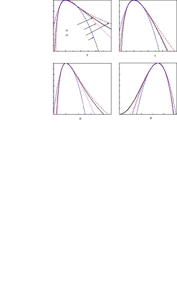
We find µ0 = 3.88. The Bayesian probability that the mean rate µ is larger than 3.88 is 10 %. Fig. 8.4 shows the likelihood functions for the two cases b = 2 and b = 0 together with the limits. For comparison are also given the likelihood ratio limits which correspond to a decrease from the maximum by e−2. (For a normal distribution this would be equivalent to two standard deviations).

We now investigate the more general case that both the acceptance ε and the background are not perfectly known, and that the p.d.f.s of the background and the acceptance fb, fε are given. For a mean Poisson signal µ the probability to observe k events is