vstatmp_engl

Fig. 8.4. Upper limits for poisson rates. The dashed lines are likelihood ratio limits (decrease by e2).

ZZ

g(k|µ) = db dε P (k|εµ + b)fb(b)fε(ε) = L(µ|k) .

For k observations this is also the likelihood function of µ. According to our scheme, we obtain the upper limit µ0 by normalization and integration,

R µ0 L(µ|k)dµ

C = R0∞ L(µ|k)dµ

0

which is solved numerically for µ0.

Example 122. Upper limit for a Poisson rate with uncertainty in background and acceptance

Observed are 2 events, expected are background events following a normal distribution N(b|2.0, 0.5) with mean value b0 = 2 and standard deviation σb = 0.5. The acceptance is assumed to follow also a normal distribution with mean ε0 = 0.5 and standard deviation σε = 0.1. The likelihood function is Z Z

L(µ|2) = dε dbP (2|εµ + b)N(ε|0.5, 0.1)N(b|2.0, 0.5) .

We solve this integral numerically for values of µ in the range of µmin = 0 to µmax = 20, in which the likelihood function is noticeable di erent from zero (see Fig. 8.5). Subsequently we determine µ0 such that the fraction C = 0.9 of the normalized likelihood function is located left of µ0. Since negative values of the normal distributions are unphysical, we cut these distributions and renormalize them. The computation in our case yields the upper limit µ0 = 7.7. In the figure we also indicate the e−2 likelihood ratio limit.

218 8 Interval Estimation

Fig. 8.5. Log-likelihood function for a Poisson signal with uncertainty in background and acceptance. The arrow indicates the upper 90% limit. Also shown is the likelihood ratio limit (decrease by e2, dashed lines).

Fig. 8.6. Renormalized likelihood function and upper limit.

8.4.4 Unphysical Parameter Values

Sometimes the allowed range of a parameter is restricted by physical or mathematical boundaries, for instance it may happen that we infer from the experimental data a negative mass. In these circumstances the parameter range will be cut and the likelihood function will be normalized to the allowed region. This is illustrated in Fig. 8.6. The integral of the likelihood in the physical region is one. The shaded area is equal to α. The parameter θ is less than θmax with confidence C = 1 − α.

We have to treat observations which are outside the allowed physical region with caution and check whether the errors have been estimated correctly and no systematic uncertainties have been neglected.

8.5 Summary

Measurements are described by the likelihood function.

•The standard likelihood ratio limits are used to represent the precision of the measurement.

•If the log-likelihood function is parabolic and the prior can be approximated by a constant, e.g. the likelihood function is very narrow, the likelihood function is proportional to the p.d.f. of the parameter, error limits represent one standard deviation and a 68.3 % probability interval.

•If the likelihood function is asymmetric, we derive asymmetric errors from the likelihood ratio. The variance of the measurement or probabilities can only be derived if the prior is known or if additional assumptions are made. The likelihood function should be published.

•Nuisance parameters are eliminated by the methods described in Chap. 7, usually using the profile likelihood.

•Error propagation is performed using the direct functional dependence of the parameters.

•Confidence intervals, upper and lower limits are computed from the normalized likelihood function, i.e. using a flat prior. These intervals usually correspond to 90% or 95% probability.

•In many cases it is not possible to assign errors or confidence intervals to parameters without making assumptions which are not uniquely based on experimental data. Then the results have to be presented such that the reader of a publication is able to insert his own assumptions and the procedure used by the author has to be documented.

9

Deconvolution

9.1 Introduction

9.1.1 The Problem

In many experiments statistical samples are distorted by limited acceptance, sensitivity, or resolution of the detectors. Is it possible to reconstruct from this distorted sample the original distribution from which the undistorted sample has been drawn?

frequency

X

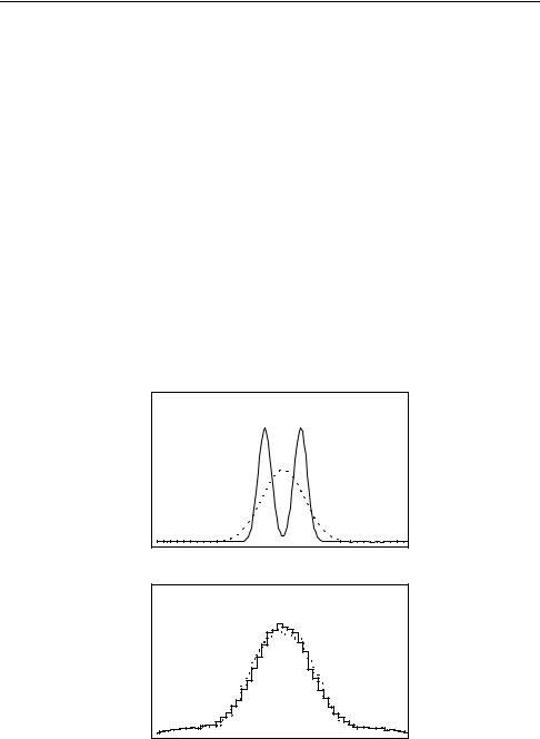
Fig. 9.1. Convolution of two di erent distributions. The distributions (top) di er hardly after the convolution (bottom).

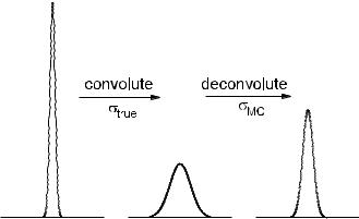
Fig. 9.2. E ect of deconvolution with a resolution wrong by 10%.

information loss. Since in realistic situations neither the sample size is infinite nor the convolution function t is known exactly, to obtain a stable result, we are forced to assume that the solution f(x) is smooth. The various deconvolution methods di er in how they accomplish the smoothing which is called regularization.

Fig. 9.1 shows two di erent original distributions and the corresponding distributions smeared with a Gaussian. In spite of extremely di erent original distributions, the distributions of the samples are very similar. This demonstrates the sizeable information loss, especially in the case of the distribution with two adjacent peaks where the convolution function is broader than the structure. Sharp structures are washed out. In case of the two peak distribution it will be di cult to reconstruct the true distribution.

Fig. 9.2 shows the e ect of using a wrong resolution function. The distribution in the middle is produced from that on the left hand side by convolution with a Gaussian with width σf . The deconvolution produces the distribution on the right

where σart2 has to be added to the squared width of the original line. Thus a Dirac δ-function becomes a normal distribution of width σart. From Table 9.1 we find that even small deviations in the resolution – e.g. estimates wrong by only 1 % – can lead to substantial artificial broadening of sharp structures. In the following parts of this chapter we will assume that the resolution is known exactly. Eventually, the corresponding uncertainties have to be evaluated by a Monte Carlo simulation.

Since statistical fluctuations prevent narrow structures in the true distribution from being resolved, we find it, vice versa, impossible to exclude artificially strongly oscillating solutions of the deconvolution problem without additional restrictions.

2249 Deconvolution

Table 9.1. E ect of di erent smearing in convolution and deconvolution.

δσart/σf

0.500.87

0.200.60

0.100.44

0.050.31

0.010.14

In the following we first discuss the common case that the observed distribution is given in the form of a histogram, and, accordingly, that a histogram should be produced by the deconvolution. Later we will consider also binning-free methods. We will assume that the convolution function also includes acceptance losses, since this does not lead to additional complications.

9.1.2 Deconvolution by Matrix Inversion

We denote the content of the bin i in the observed histogram by di, and correspondingly as θi in the true histogram. The relation 9.1 reads now

j

where the matrix element Tij gives the probability to find an event in bin i of the observed histogram which was produced in bin j of the true histogram. Of course, the relation 9.2 is valid only for expected values, the values observed in a specific

case ˆ fluctuate according to the Poisson distribution: di

In order to simplify the notation we consider in the following a one-dimensional histogram and combine the bin contents to a vector d.

If we know the histogram, i.e. the vector d, and the transfer matrix T, we get the true histogram θ by solving a set of linear equations. If both histograms have the same number of bins, that means if the matrix T is quadratic, we have simply to invert the matrix T .

Here we have to assume that T−1 exists. Without smearing and equal bin sizes in both distributions, T and T−1 are diagonal and describe acceptance losses. Often the number of bins in the true histogram is chosen smaller than in the observed one. We will come back to this slightly more complicated situation at the end of this section.

We obtain an estimate θ for the original distribution if we substitute in (9.3) the

By the usual propagation of errors we find the error matrix

226 9 Deconvolution

9.1.3 The Transfer Matrix

Until now we have assumed that we know exactly the probability Tij for observing elements in bin i which originally were produced in bin j. This is, at least in principle, impossible, as we have to average the true distribution f(x) – which we do not know

– over the respective bin interval

Therefore T depends on f. Only if f can be approximated by constants in all bins the dependence is negligible. This condition is satisfied if the width of the transfer function, i.e. the smearing, is large compared to the bin width in the true histogram. On the other hand, small bins mean strong oscillations and correlations between neighboring bins. The matrix inversion method implies oscillations. Suppressing this feature by using wide bins can lead to inconsistent results.

All methods working with histograms have to derive the transfer matrix from a smooth distribution, which is not too di erent from the true one. For methods using regularization (see below), an iteration is required, if the deconvoluted distribution di ers markedly from that used for the determination of T.

Remark: The deconvolution produces wrong results, if not all values of x′ which are used as input in the deconvolution process are covered by x values of the considered true distribution. The range in x thus has to be larger than that of x′. The safest thing is not to restrict it at all even if some regions su er from low statistics and thus will be reconstructed with marginal precision. We can eliminate these regions after the deconvolution.

In practice, the transfer matrix is usually obtained not analytically from (9.4), but by Monte Carlo simulation. In this case, the statistical fluctuations of the simulation eventually have to be taken into account. This leads to multinomial errors of the transfer matrix elements. The correct treatment of these errors is rather involved, thus, if possible, one should generate a number of simulated observations which is much larger than the experimental sample such that the fluctuations can be neglected. A rough estimate shows that for a factor of ten more simulated observations the contribution of the simulation to the statistical error of the result is only about 5% and then certainly tolerable.

9.1.4 Regularization Methods

From the above discussions it follows that it makes sense to suppress insignificant oscillations in the deconvoluted distribution. The various methods developed to achieve this, can be classified roughly as follows:

1.The deconvoluted function is processed by one of the usual smoothing procedures.

2.The true distribution is parameterized as a histogram. The parameters, i.e. the

bin contents, are fitted to the data. A regularization term Rregu is subtracted from the purely statistical log-likelihood, respectively added to the squared deviation χ2: