vstatmp_engl

5

Monte Carlo Simulation

5.1 Introduction

The possibility to simulate stochastic processes and of numerical modeling on the computer simplifies extraordinarily the solution of many problems in science and engineering. The deeper reason for this is characterized quite aptly by the German saying “Probieren geht über studieren” (Trying beats studying). Monte Carlo methods replace intellectual by computational e ort which, however, is realized by the computer.

A few simple examples will demonstrate the advantages, but also the limits of this method. The first two of them are purely mathematical integration problems which could be solved also by classical numerical methods, but show the conceptual simplicity of the statistical approach.

Example 58. Area of a circle of diameter d

We should keep in mind that without the knowledge of the quantity π the problem requires quite some mathematics but even a child can solve this problem experimentally. It may inscribe a circle into a square with edge length d, and sprinkles confetti with uniform density over it. The fraction of confetti confined inside the circle provides the area of the circle in units of the square area. Digital computers have no problem in “sprinkling confetti” homogeneously over given regions.

Example 59. Volume of the intersection of a cone and a torus

We solve the problem simply by scattering points homogeneously inside a cuboid containing the intersect. The fraction of points inside both bodies is a measure for the ratio of the intersection volume to that of the cuboid.

In the following three examples we consider the influence of the measurement process on the quantity to be determined.

Example 60. Correction of decay times

The decay time of instable particles is measured with a digital clock which is stopped at a certain maximal time. How can we determine the mean lifetime of the particles? The measured decay times are distorted by both the limited

108 5 Monte Carlo Simulation

resolution as well as by the finite measurement time, and have to be corrected. The correction can be determined by a simulation of the whole measurement process. (We will come back to details below.)

Example 61. E ciency of particle detection

Charged particles passing a scintillating fiber produce photons. A fraction of the photons is reflected at the surface of the fiber, and, after many reflections, eventually produces a signal in a photomultiplier. The photon yield per crossing particle has to be known as a function of several parameters like track length of the particle inside the fiber, its angle of incidence, fiber length and curvature, surface parameters of the fiber etc.. Here a numerical solution using classical integration methods would be extremely involved and an experimental calibration would require a large number of measurements. Here, and in many similar situations, a Monte Carlo simulation is the only sensible approach.

Example 62. Measurement of a cross section in a collider experiment

Particle experiments often consist of millions of detector elements which have to measure the trajectories of sometimes thousands of particles and the energies deposited in an enormous number of calorimeter cells. To measure a specific cross section, the corresponding events have to be selected, acceptance losses have to be corrected, and unavoidable background has to be estimated. This can only be achieved by sophisticated Monte Carlo simulations which require a huge amount of computing time. These simulations consist of two distinct parts, namely the generation of the particle reaction (event generation) which contains the interesting physics, and the simulation of the detector response. The computing time needed for the event generation is negligible compared to that required for the detector simulation. As a consequence one tries to avoid the repetition of the detector simulation and takes, if possible, modifications of the physical process into account by re-weighting events.

Example 63. Reaction rates of gas mixtures

A vessel contains di erent molecules with translational and rotational movements according to the given temperature. The molecules scatter on the walls, with each other and transform into other molecules by chemical processes depending on their energy. To be determined is the composition of the gas after a certain time. The process can be simulated for a limited number of particles. The particle trajectories and the reactions have to be computed.

All examples lead finally to integration problems. In the first three examples also numerical integration, even exact analytical methods, could have been used. For the Examples 61 and 63, however, this is hardly possible, since the number of variables is too large. Furthermore, the mathematical formulation of the problems becomes rather involved.

Monte Carlo simulation does not require a profound mathematical expertise. Due to its simplicity and transparency mistakes can be avoided. It is true, though, that the results are subject to statistical fluctuations which, however, may be kept small

enough in most cases thanks to the fast computers available nowadays. For the simulation of chemical reactions, however, (Example 63) we reach the limits of computing power quite soon, even with super computers. The treatment of macroscopic quantities (one mole, say) is impossible. Most questions can be answered, however, by simulating small samples.

Nowadays, even statistical problems are often solved through Monte Carlo simulations. In some big experiments the error estimation for parameters determined in a complex analysis is so involved that it is easier to simulate the experiment, including the analysis, several times, and to derive the errors quasi experimentally from the distribution of the resulting parameter values. The relative statistical fluctuations can be computed for small samples and then scaled down with the square root of the sample size.

In the following section we will treat the simulation of the basic univariate distributions which are needed for the generation of more complex processes. The generalization to several dimensions is not di cult. Then we continue with a short summary on Monte Carlo integration methods.

5.2 Generation of Statistical Distributions

The simplest distribution is the uniform distribution which serves as the basis for the generation of all other distributions. In the following we will introduce some frequently used methods to generate random numbers with desired distributions.

Some of the simpler methods have been introduced already in Chap. 3, Sect. 3.6.4, 3.6.5: By a linear transformation we can generate uniform distributions of any location and width. The sum of two uniformly distributed random numbers follows a triangular distribution. The addition of only five such numbers produces a quite good approximation of a Gaussian variate.

Since our computers work deterministically, they cannot produce numbers that are really random, but they can be programmed to deliver for practically any application su ciently unordered numbers, pseudo random numbers which approximate random numbers to a very good accuracy.

5.2.1 Computer Generated Pseudo Random Numbers

The computer delivers pseudo random numbers in the interval between zero and one. Because of the finite number of digits used to represent data in a computer, these are discrete, rational numbers which due to the usual floating point accuracy can take only 218 ≈ 8 · 106 di erent values, and follow a fixed, reproducible sequence which, however, appears as stochastic to the user. More refined algorithms can avoid, though, the repetition of the same sequence after 218 calls. The Mersenne twister, one of the fastest reasonable random number generators, invented in 1997 by M. Matsomoto and T. Nishimura has the enormous period of 219937 which never can be exhausted and is shown to be uniformly distributed in 623 dimensions. In all generators, the user has the possibility to set some starting value, called seed, and thus to repeat exactly the same sequence or to interrupt a simulation and to continue with the sequence in order to generate statistically independent samples.

110 5 Monte Carlo Simulation

In the following we will speak of random numbers also when we mean pseudo random numbers.

There are many algorithms for the generation of random numbers. The principle is quite simple: One performs an arithmetic operation and uses only the insignificant digits of the resulting number. How this works is shown by the prescription

xi+1 = n−1 mod(λxi; n) ,

producing from the old random number xi a new one between zero and one. The parameters λ and n fulfil the condition λ n. With the values x1 = 0.7123, λ = 4158, n = 1 we get, for instance, the number

x2 = mod(2961.7434; 1) = 0.7434 .

The apparent “randomness” is due to the cutting o the significant digits by the mod operation.

This random number generator is far from being perfect, as can be shown experimentally by investigation of the correlations of consecutive random numbers. The generators installed in the commonly used program libraries are almost always su ciently good. Nevertheless it is advisable to check their quality before starting important calculations. Possible problems with random number generators are that they have a shorter than expected repetition period, correlations of successive values and lack of uniformity. For simulations which require a high accuracy, we should remember that with the standard generators only a limited number of random numbers is available. Though intuitively attractive, randomly mixing the results of di erent random number generators does not improve the overall quality.

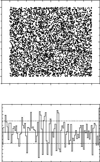
In Fig. 5.1 the values of two consecutive random numbers from a PC routine are plotted against each other. Obvious correlations and clustering cannot be detected. The histogram of a projection is well compatible with a uniform distribution. A quantitative judgment of the quality of random number generators can be derived with goodness-of-fit tests (see Chap. 10).

In principle, one could of course integrate random number generators into the computers which indeed work stochastically and replace the deterministic generators. As physical processes, the photo e ect or, even simpler, the thermal noise could be used. Each bit of a computer word could be set by a dual oscillator which is stopped by the stochastic process. Unfortunately, such hardware random number generators are presently not used, although they could be produced quite economically, presumably ≈ 103 in a single chip. They would make obsolete some discussions, which come up from time to time, on the reliability of software generators. On the other hand, the reproducibility of the random number sequence is quite useful when we want to compare di erent program versions, or to debug them.

5.2.2 Generation of Distributions by Variable Transformation

Continuous Variables

With the restrictions discussed above, we can generate with the computer random numbers obeying the uniform distribution

u(r) = 1 for 0 ≤ r ≤ 1.

112 5 Monte Carlo Simulation

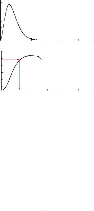
Fig. 5.2. The p.d.f (top) follows from the distribution function as indicated by the arrows.

F (x) = r,

x(r) = F −1(r) .

The variable x is calculated from the inverse function F −1 where F (x) is the distribution function which is set equal to r. For an analytic solution the p.d.f. has to be analytically integrable and the distribution function must have an inverse in analytic form.

The procedure is explained graphically in Fig. 5.2: A random number r between zero and one is chosen on the ordinate. The distribution function (or rather its inverse) then delivers the respective value of the random variable x.

In this way it is possible to generate the following distributions by simple variable transformation from the uniform distribution:

• Linear distribution:

f(x) = 2x 0 ≤ x ≤ 1 ,

√

x(r) = r .

• Power-law distribution:

f(x) = (n + 1)xn 0 ≤ x ≤ 1, n > −1 ,

x(r) = r1/(n+1) .

• Exponential distribution (Sect. 3.6.6) :

f(x) = γe−γx,

x(r) = − γ1 ln(1 − r) .

•Normal distribution (Sect. 3.6.5) : Two independent normally distributed random

numbers x, y are obtained from two uniformly distributed random numbers r1, r2, see (3.38), (3.39).

• Breit-Wigner distribution (Sect3.6.9) :

• Log-Weibull (Fisher–Tippett) distribution (3.6.12)

f(x) = exp(−x − e−x), x(r) = − ln(− ln r) .

The expression 1 − r can be replaced by r in the formulas. More general versions of these distributions are obtained by translation and/or scaling operations. A triangular distribution can be constructed as a superposition of two linear distributions. Correlated normal distributed random numbers are obtained by scaling x and y di erently and subsequently rotating the coordinate frame. How to generate superpositions of distributions will be explained in Sect. 5.2.5.

Uniform Angular, Circular and Spherical Distributions

Very often the generation of a uniform angular distribution is required. The azimuthal angle ϕ is given by

ϕ = 2πr .

To obtain a spatially isotropic distribution, we have also to generate the polar angle θ. As we have discussed in Sect. 3.5.8, its cosine is uniformly distributed in the interval [−1, 1]. Therefore

cos θ = (2r1 − 1) ,

θ = arccos(2r1 − 1) , ϕ = 2πr2 .

A uniform distribution inside a circle of radius R0 is generated by

R= R0√r1,

ϕ= 2πr2 .

114 5 Monte Carlo Simulation

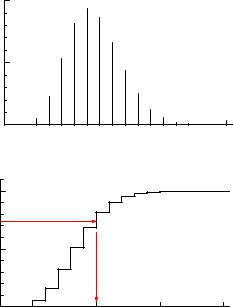
Fig. 5.3. Generation of a Poisson distributed random number.

Because the di erential area element is R dR dϕ, we have a linear distribution in R. A uniform distribution inside a sphere of radius R0 is obtained similarly from

R = R0r11/3,

θ = arccos(2r2 − 1) , ϕ = 2πr3 ,

with a quadratic distribution in R.

Discrete Distributions

The generation of random numbers drawn from discrete distributions is performed in a completely analogous fashion. We demonstrate the method with a simple example: We generate random numbers k following a Poisson distribution P (k|4.6) with expected value 4.6 which is displayed in Fig. 5.3. By summation of the bins starting from the left (integration), we obtain the distribution function S(k) = Σii=0=kP (i|4.6) shown in the figure. To a uniformly distributed random number r we attach the value k which corresponds to the minimal S(k) fulfilling S > r. The numbers k follow the desired distribution.

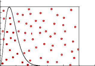
Fig. 5.4. Random selection method. The projection of the points located below the curve follow the desired distribution.

Histograms

A similar method is applied when an empirical distribution given in the form of a histogram has to be simulated. The random number r determines the bin j. The remainder r − S(j − 1) is used for the interpolation inside the bin interval. Often the bins are small enough to justify a uniform distribution for this interpolation. A linear approximation does not require much additional e ort.

For two-dimensional histograms hij we first produce a projection,

X

gi = hij ,

j

normalize it to one, and generate at first i, and then for given i in the same way j. That means that we need for each value of i the distribution summed over j.

5.2.3 Simple Rejection Sampling

In the majority of cases it is not possible to find and invert the distribution function analytically. As an example for a non-analytic approach, we consider the generation of photons following the Planck black-body radiation law. The appropriately scaled frequency x obeys the distribution

with the normalization constant c. This function is shown in Fig. 5.4 for c = 1, i.e. not normalized. We restrict ourselves to frequencies below a given maximal frequency

xmax.

A simple method to generate this distribution f(x) is to choose two uniformly distributed random numbers, where r1 is restricted to the interval (xmin, xmax) and

116 5 Monte Carlo Simulation

Fig. 5.5. Majorant (dashed) used for importance sampling.

r2 to (0, fmax). This pair of numbers P (r1, r2) corresponds to a point inside the rectangle shown in the figure. We generate points and those lying above the curve

f(x) are rejected. The density of the remaining r1 values follows the desired p.d.f. f(x).

A disadvantage of this method is that it requires several randomly distributed pairs to select one random number following the distribution. In our example the ratio of successes to trials is about 1:10. For generating photons up to arbitrary large frequencies the method cannot be applied at all.

5.2.4 Importance Sampling

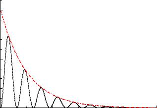
An improved selection method, called importance sampling, is the following: We look for an appropriate function m(x), called majorant, with the properties

If it exists (see Fig. 5.5), we generate x according to m(x) and, in a second step, drop stochastically for given x the fraction [m(x) − f(x)]/f(x) of the events. This means, for each event (i.e. each generated x) a second, this time uniform random number between zero and m(x) is generated, and if it is larger than f(x), the event is abandoned. The advantage is, that for m(x) being not much di erent from f(x) in most of the cases, the generation of one event requires only two random numbers. Moreover, in this way it is possible to generate also distributions which extend to infinity, as for instance the Planck distribution, and many other distributions.

We illustrate the method with a simple example (Fig. 5.5):

Example 64. Importance sampling