

vstatmp_engl
.pdf6.5 The Maximum Likelihood Method for Parameter Inference |
157 |
Weighting the Monte Carlo Observations
When we fit parameters, every parameter change obviously entails a modification of the Monte Carlo prediction. Now we do not want to repeat the full simulation with every fitting step. Apart from the fact that we want to avoid the computational e ort there is another more important reason: With the χ2 fit we find the standard error interval by letting vary χ2 by one unit. On the other hand when we compare experimental data with an optimal simulation, we expect a contribution to χ2 from the simulation of the order of p2BN/M for B histogram bins. Even with a simulation sample which is a hundred times larger than the data sample this value is of the order of one. This means that a repetition of the simulation causes considerable fluctuations of the χ2 value which have nothing to do with parameter changes. These fluctuations can only be reduced if the same Monte Carlo sample is used for all parameter values. We have to adjust the simulation to the modified parameters by weighting its observations.
Also re-weighting produces additional fluctuations. These, however, should be tolerable if the weights do not vary too much. If we are not sure that this assumption is justified, we can verify it: We reduce the number of Monte Carlo observations and check whether the result remains stable. We know that the contribution of the simulation to the parameter errors scales with the inverse square root of the number of simulated events. Alternatively, we can also estimate the Monte Carlo contribution to the error by repeating the simulation and the full estimation process.
The weights are computed in the following way: For each Monte Carlo observation x′ we know the true values x of the variates and the corresponding p.d.f. f(x|θ0) for the parameter θ0, which had been used at the generation. When we modify the parameter we weight each observation by w(θ) = f(x|θ)/f(x|θ0). The weighted distribution of x′ then describes the modified prediction.
The weighting of single observations requires a repetition of the histogramming after each parameter change. This may require too much computing time. A more e cient method is based on a Taylor expansion of the p.d.f. in powers of the parameters. We illustrate it with two examples.
Example 85. Fit of the slope of a linear distribution with Monte Carlo correction
The p.d.f. be |
1 + θx |
|
|
f(x|θ) = |
, 0 ≤ x ≤ 1 . |
||
|
|||
1 + θ/2 |
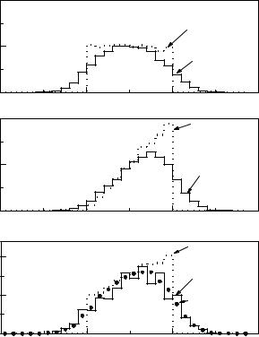
We generate observations x uniformly distributed in the interval 0 ≤ x ≤ 1, simulate the experimental resolution and the acceptance, and histogram the distorted variable x′ into bins i and obtain contents m0i. The same observations are weighted by x and summed up to the histogram m1i. These two distributions are shown in Fig. 6.10 a, b. The dotted histograms correspond to the distributions before the distortion by the measurement process. In Fig. 6.10 c is also depicted the experimental distribution. It should be possible to describe it by a superposition mi of the two Monte Carlo distributions:
di mi = m0i + θm1i . |
(6.18) |
We optimize the parameter θ such that the histogram di is described up to a normalization constant as well as possible by a superposition of the two
158 |
6 |
Parameter Inference I |
|
|
|
||
|
|
|
2000 |
a) |
|
|
|
|
|
|
|
|
|
|
|
|
|
entries |
1000 |
|
|
|
MC "true" |
|
|
|
|
|
|
||
|
|
|
|
|
|
MC folded |
|
|
|
|
|
|
|
|
|
|
|
|
0 |
-1 |
0 |
x 1 |
2 |
|
|
|
2000 |
b) |
|
|
MC "true" |
|
|
|
|
|
|
||
|
|
|
|
|
|
|
|
entries |
1000 |
|
|
|
|
|
|
|
|
|
|
|
|
|
MC folded |
|
0 |
-1 |
|
0 |
x |
1 |
2 |
|
100 |
c) |
|
|
|
MC "true" |
|
|
|
|
|
|
fitted |
||
entries |
|
|
|
|
|
|
|
50 |
|
|
|
|
|
data |
|
|
|
|
|
|
|
MC folded |
|
|
|
|
|
|
|
|
|
|
|
|
|
|
|
|
after fit |
|
0 |
-1 |
|
0 |
x |
1 |
2 |
Fig. 6.10. The superposition of two Monte Carlo distributions, a) flat and b) triangular is adjusted to the experimental data.
Monte Carlo histograms. We have to insert mi from (6.18) into (6.16) and
X set cn = N/ mi.
i
Example 86. Fit of a lifetime with Monte Carlo correction
We expand the p.d.f.
f(t|γ) = γe−γt
into a Taylor expansion at γ0 which is a first guess of the decay rate γ:
f(t|γ) = γ0e−γ0t 1 + |
Δγ |
|
Δγ |
|
γ2t2 |
|
|
(1 − γ0t) + ( |
|
)2(−γ0t + |
0 |
) + · · · . |
|
γ0 |
γ0 |
2 |
||||
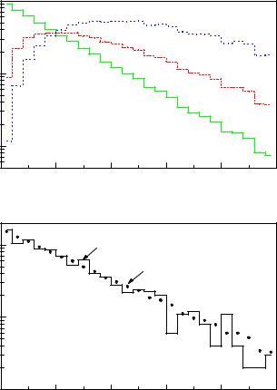
The Monte Carlo simulation follows the distribution f0 = γ0e−γ0t. Weighting the events by (1/γ0 − t) and (−t/γ0 + t2/2), we obtain the distributions f1 = (1 − γ0t)e−γ0t, f2 = (−t + γ0t2/2)e−γ0t and
f(t|γ) = f0(t) + Δγf1(t) + (Δγ)2f2(t) + · · · .
If it is justified to neglect the higher powers of Δγ/γ0, we can again describe our experimental distribution this time by a superposition of three distributions f0′ (t′), f1′ (t′), f2′ (t′) which are the distorted versions of f0, f1, f2. The
6.5 The Maximum Likelihood Method for Parameter Inference |
159 |
|
10000 |
|
|
|
|
|
a) |
|
|
|
|
|
|
2 |
|
events |
|
|
|
|
|
w = t |
|
|
|
|
|
|
w = t |
|
|
|
|
|
|
|
|
|
|
of |
1000 |
|
|
|
|
|
|
|
|
|
|
|
|
|
|
number |
|
|
|
|
|
w = 1 |
|
|
|
|
|
|
|
|
|
|
100 |
|
|
|
|
|
|
|
0 |
1 |
2 |
t |
3 |
4 |
5 |
|
100 |
|
|
|
|
|
b) |
|
|
data |
|
|
|
|
|
of events |
|
|
|
|
|
|
|
|
|
|
MC adjusted |
|
|||
|
|
|
|
|
|
|
|
number |
10 |
|
|
|
|
|
|
|
|
|
|
|
|
|
|
|
1 0 |
1 |
2 |
t |
3 |
4 |
5 |
Fig. 6.11. Lifetime fit. The dotted histogram in b) is the superposition of the three histograms of a) with weights depending on Δγ.
parameter Δγ is determined by a χ2 or likelihood fit. In our special case it is even simpler to weight f0 by t, and t2, respectively, and to superpose the corresponding distributions f0, g1 = tf0, g2 = t2f0 with the factors given in the following expression:
|
Δγ |
|
Δγ |
|
Δγ |
)2 + |
1 |
|
|
|
Δγ |
2 |
f(t|γ) = f0(t) 1 + |
|
+ γ0g1(t) |
|
+ ( |
|
|
g2 |
(t)γ02 |
|
. |
||
γ0 |
γ0 |
γ0 |
2 |
γ0 |
The parameter Δγ is then modified until the correspondingly weighted sum of the distorted histograms agrees optimally with the data. Figure 6.11 shows an example. In case the quadratic term can be neglected, two histograms are su cient.
The general case is treated in an analogous manner. The Taylor expansion is:
f(θ) = f(θ0) + Δθ |
df |
(θ0) + |
(Δθ)2 d2f |
(θ0) + · · · |
||
|
|
|
|
|||
dθ |
2! dθ2 |
|||||

160 |
6 Parameter Inference I |
|
|
|
|
|
|
|
|
|
|
|
|
|
|
|||
|
= f(θ0) 1 + Δθ |
1 df |
(Δθ)2 1 d2f |
(θ0) + · · · . |
||||||||||||||
|
|
|
|
(θ0) + |
|
|
|
|
|
|||||||||
|
f0 |
dθ |
2! f0 dθ2 |
|||||||||||||||
|
The observations x′ of the distribution f0(x|θ0) provide the histogram m0. |
|||||||||||||||||
|
Weighting with w1 and w2, where |
|
|
|
|
|
|
|||||||||||
|
|
|
|
|
1 df |
|
|
|
|
|
|
|||||||
|
w1 = |
|
|
|
|
|
(x|θ0) , |
|
||||||||||
|
f0 |
dθ |
|
|||||||||||||||
|
|
|
|
|
1 d2f |
|
|
|
|
|
|
|||||||
|
w2 = |
|
|
|
(x|θ0) , |
|
||||||||||||
|
2f0 |
dθ2 |
|
|||||||||||||||
we obtain two further histograms m1i, m2i. The parameter inference of Δθ is performed by comparing mi = (m0i+Δθm1i+Δθ2m2i) with the experimental histogram di.
In many cases the quadratic term can be omitted. In other situations it might be necessary to iterate the procedure.
6.5.10 Parameter Estimate of a Signal Contaminated by Background
In this section we will discuss point inference in the presence of background in a specific situation, where we have the chance to record independently from a signal sample also a reference sample containing pure background. The measuring times or fluxes, i.e. the relative normalization, of the two experiments are supposed to be known. The parameters searched for could be the position and width of a Breit-Wigner bump but also the slope of an angular distribution or the lifetime of a particle. The interest in this method rests upon the fact that we do not need to parameterize the background distribution and thus are independent of assumptions about its shape. This feature has to be paid for by a certain loss of precision.
The idea behind the method is simple: The log-likelihood of the wanted signal parameter as derived for the full signal sample is a superposition of the log-likelihood of the genuine signal events and the log-likelihood of the background events. The latter can be estimated from the reference sample and subtracted from the full loglikelihood.
To illustrate the procedure, imagine we want to measure the signal response of a radiation detector by recording a sample of signal heights x1, . . . , xN from a monoenergetic source. For a pure signal, the xi would follow a normal distribution with
resolution σ:
f(x|µ) = √ 1 2πσ
The unknown parameter µ is to be estimated. After removing the source, we can – under identical conditions – take a reference sample x′1, . . . , x′M of background events. They follow a distribution which is of no interest to us.
If we knew, which observations xi in our signal sample were signal (x(iS)), respec-
tively background (x(iB)) events, we could take only the S signal events and calculate the correct log-likelihood function
ln L = |
S |
ln f(x(S) µ) = |
|
|
S |
(xi(S) − µ)2 |
+ const. |
|||
Xi |
|
X |
||||||||
|
|
i | |
|
− |
2σ2 |
|
|
|||
|
=1 |
|
|
i=1 |
|
|
||||
|
|
|
|
|
|
|
|
|||
= |
N |
(xi − µ)2 |
+ |
B |
|
(xi(B) − µ)2 |
+ const. , |
|||
Xi |
|
|
||||||||
|
2σ2 |
X |
|
2σ2 |
|
|
||||
|
− |
|
|
i=1 |
|
|
|
|||
|
=1 |
|
|
|
|
|
|
|||

6.5 The Maximum Likelihood Method for Parameter Inference |
161 |
with S + B = N. The second unknown term can be estimated from the control sample
B |
(xi(B) − µ)2 |
M |
(xi′ − µ)2 |
. |
X |
|
|||
2σ2 ≈ |
Xi |
|||
i=1 |
=1 |
2σ2 |
||
|
|
|
||
The logarithm of our corrected log-likelihood becomes:
ln L˜ = |
|
N |
(xi − µ)2 |
+ |
M |
(xi′ − µ)2 |
. |
|
|
X |
|||||
|
− |
Xi |
2σ2 |
||||
|
=1 |
2σ2 |
i=1 |
||||
|
|
|
|
|
|
||
We call it pseudo log-likelihood, ˜, to distinguish it from a genuine log-likelihood. ln L
To obtain the estimate µˆ of our parameter, we look for the parameter µˆ which
maximizes ˜ and find the expected simple function of the mean values , ′: ln L x x
|
P |
|
N − P |
M |
||||
|
|
|
N |
|||||
µˆ = |
|
|
i=1 xi − |
i=1 x′ |
|
|||
|
|
|
|
M |
|
|||
|
|
|
|
|
|
|
||
|
|
|
|
|
|
|
||
|
N |
|
|
− Mx′ |
. |
|
|
|
= |
x |
(6.19) |
||||||
|
|
|
||||||
|
N − M |
|
|
|||||
The general problem where the sample and parameter spaces could be multidimensional and with di erent fluxes of the signal and the reference sample, is solved in complete analogy to our example: Given a contaminated signal distribution of size N and a reference distribution of size M and flux 1/r times larger than that of the signal sample, we put
|
N |
M |
|
ln L˜ |
Xi |
X |
(6.20) |
= |
ln f(xi|θ) − r ln f(xi′ |θ) . |
||
|
=1 |
i=1 |
|
For small event numbers, for example if the flux-corrected number of background events in the reference sample exceeds the total number of events in the main sample,
, it may happen that ˜ becomes un-bounded from above (for instance rM > N ln L
asymptotically a parabola opening to the upper side), rendering a maximum undefined.
The formula (6.20) is completely general and does not depend on the shape of the background distribution8. It avoids histogramming which is problematic for low event counts. Especially, those methods which subtract a background histogram from the signal histogram often fail in such a situation. A di erent method, where the shape of the background distribution is approximated by probability density estimation (PDE) will be given in Sect. 12.1.1.
To get a feeling of the uncertainty of the corrected estimate, we return to our example and look at the di erence of the estimate µˆ from the uncontaminated estimate x(S) which we can set without loss of generality equal to zero. From simple error propagation we find:
=Bx(B) − Mx′ . S + B − M
8The method which we present in this section has been taken from the Russian translation of the book by Eadie et al. [6] and has been introduced probably by the Russian editors [32].
162 6 Parameter Inference I
number of events
|
signal sample |
|
|
||
30 |
|
|
|
|
|
20 |
|
|
|
|
|
10 |
|
|
|
|
|
0 |
-4 |
-2 |
0 |
2 |
4 |
|
|||||
|
|
|
x |
|
|
background
30 reference sample
20 |
|
|
|
|
10 |
|
|
|
|
0-4 |
-2 |
0 |
2 |
4 |
|
|
x |
|
|
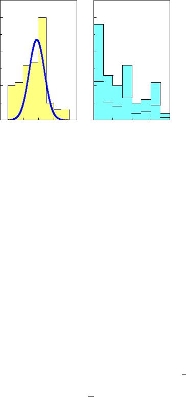
Fig. 6.12. Experimental distribution of a normally distributed signal over background (left) and background reference sample (right). The lower histogram is scaled to the signal flux.
Without going into the details, we realize that the error increases i) with the amount of background, ii) with the di erence of the expected value of the reference distri-
bution from that of the genuine signal distribution, and iii) with the variance of |
|||||||||
the background distribution. Correspondingly, we have to require |
√ |
|
|||||||
2M S, more |
|||||||||
specifically |
√ |
√ |
√ |
|
estimate of |
||||
2M|µB − µS | Sσ and |
2MσB Sσ. Here |
2M is an 2 1/2 |
|
||||||
the Poisson error of B − M, S ≈ N − M, µB ≈ |
x′ |
, µS ≈ µˆ, σB ≈ (x′2 − |
x |
) |
. |
||||
Also this consideration can be generalized: Stated qualitatively, the contribution to the parameter uncertainty is small, if background and signal lead to similar parameter estimates, if the background estimate has a small uncertainty, and, trivially, if the amount of background is small. This applies also, for instance, when we estimate the asymmetry parameter of an angular distribution contaminated by background.
The shape itself of the pseudo likelihood cannot be used directly to estimate the parameter errors. The calculation of the error in the asymptotic approximation is given in Appendix 13.4.
An alternative procedure for the error estimation is the bootstrap method, where we take a large number of bootstrap samples from the experimental distributions of both the signaland the control experiment and calculate the background corrected parameter estimate for each pair of samples, see Chap. 12.2.
Example 87. Signal over background with background reference sample
Fig. 6.12 shows an experimental histogram of a normally distributed signal of width σ = 1 contaminated by background, together 95 events with mean x = 0.61 and empirical variance v2 = 3.00. The right hand side is the distribution of a background reference sample with 1/r = 2.5 times the flux of the signal sample, containing 91 events with mean x′ = −1.17 and variance v′2 = 4.79.

6.6 Inclusion of Constraints |
163 |
The mean of the signal is obtained from the flux corrected version of (6.19):
µˆ = Nx − rMx′ N − rM
= 95 · 0.61 − 0.4 · 91 · 1.17 = −0.26 ± 0.33 . 95 − 0.4 · 91
The error is estimated by linear error propagation. The result is indicated in Fig. 6.12. The distributions were generated with nominally 60 pure signal plus 40 background events and 100 background reference events. The signal corresponds to a normal distribution, N(x|0, 1), and the background to an exponential, exp(−0.2x).
6.6 Inclusion of Constraints
6.6.1 Introduction
The interesting parameters are not always independent of each other but are often connected by constraint equations like physical or geometrical laws.
As an example let us look at the decay of a Λ particle into a proton and a pion, Λ → p + π, where the direction of flight of the Λ hyperon and the momentum vectors of the decay products are measured. The momentum vectors of the three particles which participate in the reaction are related through the conservation laws of energy and momentum. Taking into account the conservation laws, we add information and can improve the precision of the momentum determination.
In the following we assume that we have N direct observations xi which are predicted by functions ti(θ) of a parameter vector θ with P components as well as K constraints of the form hk(θ1, . . . , θP ) = 0. Let us assume further that the uncertainties i of the observations are normally distributed and that the constraints are fulfilled with the precision δk,
k |
1 |
P |
|
(ti(θ) − xi)2 |
|
||
|
|
|
|
h2 |
(θ , . . . , θ ) |
|
|
then χ2 can be written in the form:
χ2 = XN [xi − ti(θ)]2
2 i=1 i
=2i ,
=δk2 ,
|
K h2 |
(θ) |
|
||
+ |
|
k |
|
|
. |
|
δ2 |
||||
X
k=1 k
(6.21)
(6.22)
We minimize χ2 by varying the parameters and obtain their best estimates at the minimum of χ2. This procedure works also when the constraints contain more than
Nparameters, as long as their number P does not exceed the sum N + K. A corresponding likelihood fit would maximize
N |
1 |
K |
h2 |
(θ) |
||
X |
ln f(xi|θ) − |
|
X |
k |
|
. |
ln L = |
2 |
k=1 |
δk2 |
|||
i=1 |
|
|
|
|
|
|
In most cases the constraints are obeyed exactly, δk = 0, and the second term in (6.22) diverges. This di culty is avoided in the following three procedures:

164 6 Parameter Inference I
1.The constraints are used to reduce the number of parameters.
2.The constraints are approximated by narrow Gaussians.
3.Lagrange multipliers are adjusted to satisfy the constraints.
We will discuss the problem in terms of a χ2 minimization. The transition to a likelihood fit is trivial.
6.6.2 Eliminating Redundant Parameters
Sometimes it is possible to eliminate parameters by expressing them by an unconstrained subset.
Example 88. Fit with constraint: two pieces of a rope
A rope of exactly 1 m length is cut into two pieces. A measurement of both pieces yields l1 = 35.3 cm and l2 = 64.3 cm, both with the same Gaussian
|
|
|
|
ˆ |
ˆ |
of the lengths. |
uncertainty of δ = 0.3. We have to find the estimates λ1 |
, λ2 |
|||||
We minimize |
(l1 − λ1)2 |
|
(l2 − λ2)2 |
|
|
|
χ2 = |
+ |
|
|
|
||
δ2 |
δ2 |
|
|
|||
|
|
|
|
|||
including the constraint λ1 + λ2 = L = 100 cm. We simply replace λ2 by L − λ1 and adjust λ1, minimizing
χ2 = |
(l1 − λ1)2 |
+ |
(L − l2 − λ1)2 |
. |
|
δ2 |
|
δ2 |
|
The minimization relative to λ1 leads to the result:
λˆ |
= |
L |
+ |
l1 − l2 |
|
= 35.5 |
± |
0.2 cm |
|
|
2 |
|
|
|
|||||||
1 |
|
2 |
|
|
|
|
|
|||
and the corresponding estimate of λ2 |
is just the complement of |
ˆ |
with |
|||||||
λ1 |
||||||||||
respect to the full length. Note that due to the constraint the error of λi |
|
is reduced by a factor |
√ |
2, as can easily be seen from error propagation. |
|
The constraint has the same e ect as a double measurement, but with the modification that now the results are (maximally) anti-correlated: one finds cov(λ1λ2) = −var(λi).
Example 89. Fit of the particle composition of an event sample
A particle identification variable x has di erent distributions fi(x) for di erent particles. The p.d.f. given the relative particle abundance λm for particle species m out of M di erent particles is
|
M |
|
|
f(x|λ1, . . . , λM ) = X λmfm(x) , |
|
||
X |
m=1 |
|
|
λm = 1 . |
(6.23) |
||
|
|||
As the constraint relation is linear, we can easily eliminate the parameter λM to get rid of the constraint P λm = 1:
|
|
|
6.6 Inclusion of Constraints 165 |
|
|
|
M−1 |
|
M−1 |
|
|
X |
|
X |
fM−1(x|λ1, . . . , λM−1) = |
λmfm(x) + (1 − λm)fM (x) . |
|||
|
|
m=1 |
|
m=1 |
The log-likelihood for N particles is |
|
|
||
ln L = N ln |
"M−1 |
λmfm(xi) + (1 − M−1 |
λm)fM (xi)# . |
|
Xi |
X |
|
X |
|
=1 |
m=1 |
|
m=1 |
|
From the MLE we obtain in the usual way the first M −1 parameters and their error matrix E. The remaining parameter λM and the related error matrix elementsPeMj are derived from the constraint (6.23) and the corresponding relation Δλm = 0. The diagonal error is the expected value of (ΔλM )2:
|
M−1 |
|
|
ΔλM = − |
X |
|
|
Δλm , |
|
||
|
m=1 |
|
|
M−1 |
2 |
|
|
|
|
||
|
X |
|
|
(ΔλM )2 = "m=1Δλm# |
, |
|
|
M−1 |
M−1M−1 |
||
X |
X X |
||
EMM = |
Emm + |
|
Eml . |
m=1 |
m |
l6=m |
|
|
|
|
|
The remaining elements are computed analogously:
MX−1
EMj = EjM = −Ejj − Emj . m6=j
An iterative method, called channel likelihood, to find the particle contributions, is given in [34].
These trivial examples are not really representative for the typical problems we have to solve in particleor astrophysics. Indeed, it is often complicated or even impossible to reduce the parameter set analytically to an unconstrained subset. But we can introduce a new unconstrained parameter set which then predicts the measured quantities. To find such a set is straight forward in the majority of problems: We just have to think how we would simulate the corresponding experimental process. A simulation is always based on a minimum set of parameters. Constraints are obeyed automatically.
Example 90. Kinematical fit with constraints: eliminating parameters
A neutral particle c is decaying into two charged particles a and b, for instance Λ → p + π−. The masses mc, ma, mb are known. Measured are the momenta πa, πb of the decay products and the decay vertex ρ. The measurements of the components of the momentum vectors are correlated. The inverse error matrices be Va and Vb. The origin of the decaying particle be at the origin of the coordinate system. Thus we have 9 measurements (r, pa, pb), 10 parameters, namely the 3 momentum vectors and the distance (πc, πa, πb, ρ), and 4 constraints from momentum and energy conservation:

166 6 Parameter Inference I
π(πc, πa, πb) ≡ πc − πa − πb = 0 , |
|
− q |
|
|
|
|
||||||||
ε(πc, πa, πb) ≡ p |
|
|
|
− p |
|
|
πb2 − mb2 |
= 0 . |
||||||
πc2 + mc2 |
πa2 + ma2 |
|||||||||||||
The χ2 expression is |
|
|
|
|
|
|
|
|
|
|
|
|
|
|
3 |
|
|
2 |
3 |
|
|
|
|
|
|
|
|
|
|
X |
ri − ρi |
|
X |
|
|
|
|
|
|
|
|
|
||
χ2 = |
|
+ |
|
|
(p |
ai − |
π )V (p |
aj − |
π ) + |
|||||
i=1 |
δri |
|
i,j=1 |
|
ai aij |
aj |
||||||||
X3
+(pbi − πbi)Vbij (pbj − πbj ) .
i,j=1
The vertex parameters ρi are fixed by the vector relation ρ = ρπc/|πc|. Now we would like to remove 4 out of the 10 parameters using the 4 constraints.
A Monte Carlo simulation of the Λ decay would proceed as follows: First we would select the Λ momentum vector (3 parameters). Next the decay length would be generated (1 parameter). The decay of the Λ hyperon into proton and pion is fully determined when we choose the proton direction in the lambda center of mass system (2 parameters). All measured laboratory quantities and thus also χ2 can then be expressed analytically by these 6 unconstrained quantities (we omit here the corresponding relations) which are varied in the fitting procedure until χ2 is minimal. Of course in the fit we would not select random starting values for the parameters but the values which we compute from the experimental decay length and the measured momentum vectors. Once the reduced parameter set has been adjusted, it is easy to compute also the remaining laboratory momenta and their errors which, obviously, are strongly correlated.
Often the reduced parameter set is more relevant than the set corresponding to the measurement, because a simulation usually is based on parameters which are of scientific interest. For example, the investigation of the Λ decay might have the goal to determine the Λ decay parameter which depends on the center of mass direction of the proton relative to the Λ polarization, i.e. on one of the directly fitted quantities.
6.6.3 Gaussian Approximation of Constraints
As suggested by formula (6.22) to fulfil the constraints within the precision of our measurement, we just have to choose the uncertainty δk su ciently small. We will give a precise meaning to the expression su ciently small below.
Example 91. Example 88 continued
Minimizing
χ2 = |
(l1 − λ1)2 |
+ |
(l2 − λ2)2 |
+ |
(λ1 + λ2 − L)2 |
. |
|
δ2 |
|
δ2 |
|
(10−5δ)2 |
|
produces the same result as the fit presented above. The value δk2 = 10−10δ2 is chosen small compared to δ.