vstatmp_engl

Fig. 10.7. Critical χ2 values as a fnction of the number of degrees of freedom with the significance level as parameter.

The χ2 comparison becomes a test, if we accept the theoretical description of the data only if the p-value exceeds a critical value, the significance level α, and reject it for p < α. The χ2 test is also called Pearson test after the statistician Karl Pearson who has introduced it already in 1900.

Figure 10.7 gives the critical values of χ2, as a function of the number of degrees of freedom with the significance level as parameter. To simplify the presentation we have replaced the discrete points by curves. The p-value as a function of χ2 with NDF as parameter is available in the form of tables or in graphical form in many books. For large f, about f > 20, the χ2 distribution can be approximated su ciently well by a normal distribution with mean value x0 = f and variance s2 = 2f. We are then able to compute the p-values from integrals over the normal distribution. Tables can be found in the literature or alternatively, the computation can be performed with computer programs like Mathematica or Maple.

The Choice of Binning

There is no general rule for the choice of the number and width of the histogram bins for the χ2 comparison but we note that the χ2 test looses significance when the number of bins becomes too large.

To estimate the e ect of fine binning for a smooth deviation, we consider a systematic deviation which is constant over a certain region with a total number of entries N0 and which produces an excess of εN0 events. Partitioning the region into B bins would add to the statistical χ2 in each single bin the contribution:

χ2 = (εN0/B)2 = ε2N0 . s N0/B B

For B bins we increase χ2 by ε2N0 which is to be compared to the purely statistical

It decreases with the square root of the number of bins.

We recommend a fine binning only if deviations are considered which are restricted to narrow regions. This could be for instance pick-up spikes. These are pretty rare in our applications. Rather we have systematic deviations produced by non-linearity of measurement devices or by background and which extend over a large region. Then wide intervals are to be preferred.

In [58] it is proposed to choose the number of bins according to the formula B = 2N2/5 as a function of the sample size N.

Example 127. Comparison of di erent tests for background under an exponential distribution

In Fig. 10.2 a histogrammed sample is compared to an exponential. The sample contains, besides observations following this distribution, a small contribution of uniformly distributed events. From Table 10.1 we recognize that this defect expresses itself by small p-values and that the corresponding decrease becomes more pronounced with decreasing number of bins.

Some statisticians propose to adjust the bin parameters such that the number of events is the same in all bins. In our table this partitioning is denoted by e.p. (equal probability). In the present example this does not improve the significance.

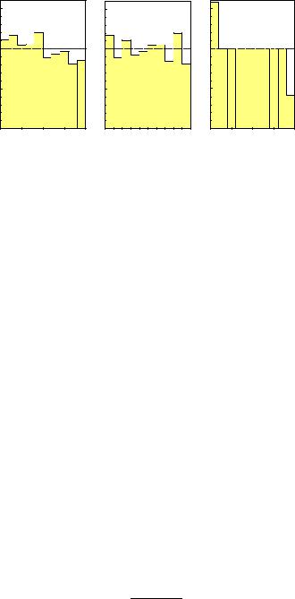
The value of χ2 is independent of the signs of the deviations. However, if several adjacent bins show an excess (or lack) of events like in the left hand histogram of Fig. 10.8 this indicates a systematic discrepancy which one would not expect at the same level for the central histogram which produces the same value for χ2. Because correlations between neighboring bins do not enter in the test, a visual inspection is often more e ective than the mathematical test. Sometimes it is helpful to present

a hyperplane containing the origin, of the N-dimensional z-space. Consequently, the distance in z-space is confined to this subspace and derived from N − 1 components. For Z free parameters we get Z constraints and a (N −Z)-dimensional subspace. The independent components (dimensions) of this subspace are called degrees of freedom. The number of degrees of freedom is f = N − Z as pretended above. Obviously, the sum of f squared components will follow a χ2 distribution with f degrees of freedom.

In the case of fitting a normalized distribution to a histogram with B bins which we have considered above, we had to set (see Sect. 3.6.7) f = B −1. This is explained by a constraint of the form z1 + · · · + zB = 0 which is valid due to the equality of the normalization for data and theory.

The χ2 Test for Small Samples

When the number of entries per histogram bin is small, the approximation that the variations are normally distributed is not justified. Consequently, the χ2 distribution should no longer be used to calculate the p-value.

Nevertheless we can use in this situation the sum of quadratic deviations χ2 as test statistic. The distribution f0(χ2) has then to be determined by a Monte Carlo simulation. The test then is slightly biased but the method still works pretty well.

Warning

The assumption that the distribution of the test statistic under H0 is described by a χ2 distribution relies on the following assumptions: 1. The entries in all bins of the histogram are normality distributed. 2. The expected number of entries depends linearly on the free parameters in the considered parameter range. An indication for a non-linearity are asymmetric errors of the adjusted parameters. 3. The estimated uncertainties σi in the denominators of the summands of χ2 are independent of the parameters. Deviations from these conditions a ect mostly the distribution at large values of χ2 and thus the estimation of small p-values. Corresponding conditions have to be satisfied when we test the GOF of a curve to measured points. Whenever we are not convinced about their validity we have to generate the distribution of χ2 by a Monte Carlo simulation.

10.3.4 The Likelihood Ratio Test

General Form

The likelihood ratio test compares H0 to a parameter dependent alternative H1 which includes H0 as a special case. The two hypothesis are defined through the p.d.f.s f(x|θ) and f(x|θ0) where the parameter set θ0 is a subset of θ, often just a fixed value of θ. The test statistic is the likelihood ratio λ, the ratio of the likelihood of H0 and the likelihood of H1 where the parameters are chosen such that they maximize the likelihoods for the given observations x. It is given by the expression

262 10 Hypothesis Tests

or equivalently by

ln λ = sup ln L(θ0|x) − sup ln L(θ|x) .

If θ0 is a fixed value, this expression simplifies to ln λ = ln L(θ0|x) − sup ln L(θ|x). From the definition (10.7) follows that λ always obeys λ ≤ 1.

Example 129. Likelihood ratio test for a Poisson count

Let us assume that H0 predicts µ0 = 10 decays in an hour, observed are 8. The likelihood to observe 8 for the Poisson distribution is L0 = P (8|10) = e−10108/8!. The likelihood is maximal for µ = 8, it is L = P (8|8) = e−888/8! Thus the likelihood ratio is λ = P (8|10)/P (8|8) = e−2(5/4)8 = 0.807. The probability to observe a ratio smaller than or equal to 0.807 is

µ0 = 10 are given in Table 10.3 It is seen, that the sum over k runs over

Table 10.3. Values of λ and P , see text.

all k, except k = 9, 10, 11, 12: p = Σk8=0P (k|10) + Σk∞=13P (k|10) = 1 −

Σk12=9P (k|10) = 0.541 which is certainly acceptable. This is an example for the p-value of a two-sided test.

The likelihood ratio test in this general form is useful to discriminate between a specific and a more general hypothesis, a problem which we will study in Sect. 10.5.2. To apply it as a goodness-of-fit test, we have to histogram the data.

The Likelihood Ratio Test for Histograms

Q

We have shown that the likelihood L0 = i f0(xi) of a sample cannot be used as a test statistic, but when we combine the data into bins, a likelihood ratio can be defined for the histogram and used as test quantity. The test variable is the ratio of the likelihood for the hypothesis that the bin content is predicted by H0 and the likelihood for the hypothesis that maximizes the likelihood for the given sample. The latter is the likelihood for the hypothesis where the prediction for the bin coincides with its content. If H0 is not simple, we take the ratio of the maximum likelihood allowed by H0 and the unconstrained maximum of L.

For a bin with content d, prediction t and p.d.f. f(d|t) this ratio is λ = f(d|t)/f(d|d) since at t = d the likelihood is maximal. For the histogram we have to multiply the ratios of the B individual bins. Instead we change to the log-likelihoods and use as test statistic

XB

V = ln λ = [ln f(di|ti) − ln f(di|di)] .

i=1

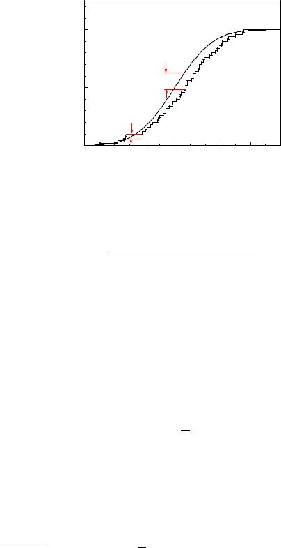
Fig. 10.10. P-value as a function of the Kolmogorov test statistic D .

The Kolmogorov–Smirnov test emphasizes more the center of the distribution than the tails because there the distribution function is tied to the values zero and one and thus is little sensitive to deviations at the borders. Since it is based on the distribution function, deviations are integrated over a certain range. Therefore it is not very sensitive to deviations which are localized in a narrow region. In Fig. 10.8 the left hand and the right hand histograms have the same excess of entries in the region left of the center. The Kolmogorov–Smirnov test produces in both cases approximately the same value of the test statistic, even though we would think that the distribution of the right hand histogram is harder to explain by a statistical fluctuation of a uniform distribution. This shows again, that the power of a test depends strongly on the alternatives to H0. The deviations of the left hand histogram are well detected by the Kolmogorov–Smirnov test, those of the right hand histogram much better by the Anderson–Darling test which we will present below.

There exist other EDF tests [57], which in most situations are more e ective than the simple Kolmogorov–Smirnov test.

10.3.6 Tests of the Kolmogorov–Smirnov – and Cramer–von Mises

Families

In the Kuiper test one uses as the test statistic the sum V = D+ + D− of the two deviations of the empirical distribution function S from F . This quantity is designed for distributions “on the circle”. This are distributions where the beginning and the end of the distributed quantity are arbitrary, like the distribution of the azimuthal angle which can be presented with equal justification in all intervals [ϕ0, ϕ0 + 2π] with arbitrary ϕ0.

The tests of the Cramer–von Mises family are based on the quadratic di erence between F and S. The simple Cramer–von Mises test employs the test statistic

266 10 Hypothesis Tests

Z ∞

W 2 = [(F (x) − S(x)]2 dF .

−∞

In most situations the Anderson–Darling test with the test statistic A2 and the test of Watson with the test statistic U2

are superior to the Kolmogorov–Smirnow test.

The test of Anderson emphasizes especially the tails of the distribution while Watson’s test has been developed for distributions on the circle. The formulas above look quite complicated at first sight. They simplify considerably when we perform a probability integral transformation (PIT ). This term stands for a simple transformation of the variate x into the variate z = F0(x), which is uniformly distributed in the interval [0, 1] and which has the simple distribution function H0(z) = z. With the transformed step distribution S (z) of the sample we get

In the Appendix 13.7 we show how to compute the test statistics. There also the asymptotic distributions are collected.

10.3.7 Neyman’s Smooth Test

This test [59] is di erent from those discussed so far in that it parameterizes the alternative hypothesis. Neyman introduced the smooth test in 1937 (for a discussion by E. S. Pearson see [60]) as an alternative to the χ2 test, in that it is insensitive to deviations from H0 which are positive (or negative) in several consecutive bins. He insisted that in hypothesis testing the investigator has to bear in mind which departures from H0 are possible and thus to fix partially the p.d.f. of the alternative. The test is called “smooth” because, contrary to the χ2 test, the alternative hypothesis approaches H0 smoothly for vanishing parameter values. The hypothesis under test H0 is again that the sample after the PIT, zi = F0(xi), follows a uniform distribution in the interval [0, 1].

The smooth test excludes alternative distributions of the form

where θi are parameters and the functions πi(z) are modified orthogonal Legendre polynomials that are normalized to the interval [0, 1] and symmetric or antisymmetric with respect to z = 1/2: