vstatmp_engl

The Sample Median

A first step (already proposed by Laplace) in the direction to estimators more robust than the sample mean is the introduction of the sample median as estimator for location parameters. While the former follows to an extremely outlying observation up to ±∞, the latter stays nearly unchanged in this case. This change can be expressed as a change of the object function, i.e. the function to be minimized with respect to µ, from Pi(yi − µ)2 to Pi |yi − µ| which is indeed minimized if µˆ coincides with the sample median in case of N odd. For even N, µˆ is the mean of the two innermost points. Besides the slightly more involved computation (sorting instead of summing), the median is not an optimal estimator for a pure Gaussian distribution:

var(median) = π2 var(mean) = 1.571 var(mean) ,

but it weights large residuals less and therefore performs better than the arithmetic mean for distributions which have longer tails than the Gaussian. Indeed for large N we find for the Cauchy distribution var(median) = π2/(4N), while var(mean) = ∞ (see 3.6.9), and for the two-sided exponential (Laplace) distribution var(median) = var(mean)/2.

with ρ(z) = z2 for the LS method which is optimal for Gaussian errors. For the Laplace distribution mentioned above the optimal object function is based on ρ(z) = |z|, derived from the likelihood analog which suggests ρ ln f. To obtain a more robust estimation the function ρ can be modified in various ways but we have to retain the symmetry, ρ(z) = ρ(−z) and to require a single minimum at z = 0. This kind of estimators with object functions ρ di erent from z2 are called M-estimators, “M” reminding maximum likelihood. The best known example is due to Huber, [92]. His proposal is a kind of mixture of the appropriate functions of the Gauss and the Laplace cases:

The constant c has to be adapted to the given problem. For a normal population the estimate is of course not e cient. For example with c = 1.345 the inverse of the variance is reduced to 95% of the standard value. Obviously, the fitted object function (13.38) no longer follows a χ2 distribution with appropriate degrees of freedom.

Estimators with High Breakdown Point

In order to compare di erent estimators with respect to their robustness, the concept of the breakdown point has been introduced. It is the smallest fraction ε of corrupted data points which can lead the fitted values to di er by an arbitrary large amount

378 13 Appendix

from the correct ones. For LS, ε approaches zero, but for M-estimators or truncated fits, changing a single point would be not su cient to shift the fitted parameter by a large amount. The maximal value of ε is smaller than 50% if the outliers are the minority. It is not di cult to construct estimators which approach this limit, see [93]. This is achieved, for instance, by ordering the residuals according to their absolute value (or ordering the squared residuals, resulting in the same ranking) and retaining only a certain fraction, at least 50%, for the minimization. This so-called least trimmed squares (LTS) fit is to be distinguished from truncated least square fit (LST, LSTS) with a fixed cut against large residuals.

An other method relying on rank order statistics is the so-called least median of

squares (LMS) method . It is defined as follows: Instead of minimizing with respect

P

to the parameters µ the sum of squared residuals, i ri2, one searches the minimum of the sample median of the squared residuals:

minimizeµ median(ri2(µ)) .

This definition implies that for N data points, N/2 + 1 points enter for N even and (N + 1)/2 for N odd. Assuming equal errors, this definition can be illustrated geometrically in the one-dimensional case considered here: µˆ is the center of the smallest interval (vertical strip in Fig. 13.9) which covers half of all x values. The width 2 of this strip can be used as an estimate of the error. Many variations are of course possible: Instead of requiring 50% of the observations to be covered, a larger fraction can be chosen. Usually, in a second step, a LS fit is performed with the retained observations, thus using the LMS only for outlier detection. This procedure is chosen, since it can be shown that, at least in the case of normal distributions, ranking methods are statistically inferior as compared to LS fits.

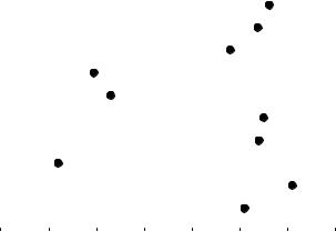
Example 155. Fitting a mean value in presence of outliers

In Fig.13.9 a simple example is presented. Three data points, representing the outliers, are taken from N(3, 1) and seven from N(10, 1). The LS fit (7.7±1.1) is quite disturbed by the outliers. The sample median is here initially 9.5, and becomes 10.2 after excluding the outliers. It is less disturbed by the outliers. The LMS fit corresponds to the thick line, and the minimal strip of width 2 to the dashed lines. It prefers the region with largest point density and is therefore a kind of mode estimator. While the median is a location estimate which is robust against large symmetric tails, the mode is also robust against asymmetric tails, i.e. skew distributions of outliers.

A more quantitative comparison of di erent fitting methods is presented in Table 13.1. We have generated 100000 samples with a 7 point signal given by N(10, 1) and 3 points of background, a) asymmetric: N(3, 1) (the same parameters as used in the example before), b) uniform in the interval [5, 15], and in addition c) pure normally distributed points following N(10, 1) without background. The table contains the root mean squared deviation of the mean values from the nominal value of 10. To make the comparison fair, as in the LMS method also in the trimmed LS fit 6 points have been retained and in the sequentially truncated LS fit a minimum of 6 points was used.

With the asymmetric background, the first three methods lead to biased mean values (7.90 for the simple LS, 9.44 for the median and 9.57 for the trimmed LS) and thus the corresponding r.m.s. values are relatively large. As expected the median su ers much less from the background than a stan-

Fig. 13.9. Estimates of the location parameter for a sample with three outliers.

Table 13.1. Root mean squared deviation of di erent estimates from the nominal value.

dard LS fit. The results of the other two methods, LMS and LS sequentially truncated perform reasonable in this situation, they succeed to eliminate the background completely without biasing the result but are rather weak when little or no background is present. The result of LMS is not improved in our example when a least square fit is performed with the retained data.

The methods can be generalized to the multi-parameter case. Essentially, the r.m.s deviation is replaced by χ2. In the least square fits, truncated or trimmed, the measurements with the larges χ2 values are excluded. The LMS method searches for the parameter set where the median of the χ2 values is minimal.

More information than presented in this short and simplified introduction into the field of robust methods can be found in the literature cited above and the newer book of R. Maronna, D. Martin and V. Yohai [91].

References

1.M. G. Kendall and W. R. Buckland, A Dictionary of Statistical Terms, Longman, London (1982).

2.M. G. Kendall and A. Stuart, The Advanced Theory of Statistics, Gri n, London (1979).

3.S. Brandt, Data Analysis, Springer, Berlin (1999).

4.A. G. Frodesen, O. Skjeggestad, M. Tofte, Probability and Statistics in Particle Physics, Universitetsforlaget, Bergen (1979).

5.L. Lyons, Statistics for Nuclear and Particle Physicists, Cambridge University Press (1992).

6.W. T. Eadie et al., Statistical Methods in Experimental Physics, North-Holland, Amsterdam, (1982).

7.F. James, Statistical Methods in Experimental Physics, World Scientific Publishing, Singapore (2007).

8.V. Blobel, E. Lohrmann, Statistische und numerische Methoden der Datenanalyse, Teubner, Stuttgart (1998).

9.B. P. Roe, Probability and Statistics in Experimental Physics, Springer, Berlin (2001).

10.R. Barlow, Statistics, Wiley, Chichester (1989).

11.G. Cowan, Statistical Data Analysis, Clarendon Press, Oxford (1998).

12.G. D’Agostini, Bayesian Reasoning in Data Analysis: A Critical Introduction, World Scientific Pub., Singapore (2003).

13.T. Hastie, R. Tibshirani, J. H. Friedman, The Elements of Statistical Learning, Springer, Berlin (2001).

14.G. E. P. Box and G. C. Tiao, Bayesian Inference in Statistical Analysis, AddisonWeseley, Reading (1973).

15.R. A. Fisher, Statistical Methods, Experimental Design and Scientific Inference, Oxford University Press (1990). (First publication 1925).

16.A. W. F. Edwards, Likelihood, The John Hopkins University Press, Baltimore (1992).

17.I. J. Good, Good Thinking, The Foundations of Probability and its Applications, Univ. of Minnesota Press, Minneapolis (1983).

18.L. J. Savage, The Writings of Leonard Jimmie Savage - A Memorial Selection, ed. American Statistical Association, Washington (1981).

19.H. Je reys, Theory of Probability, Clarendon Press, Oxford (1983).

20.L. J. Savage, The Foundation of Statistical Inference, Dover Publ., New York (1972).

21.Proceedings of PHYSTAT03, Statistical Problems in Particle Physics, Astrophysics and Cosmology ed. L. Lyons et al., SLAC, Stanford (2003) Proceedings of PHYSTAT05,

Statistical Problems in Particle Physics, Astrophysics and Cosmology ed. L. Lyons et al., Imperial College Press, Oxford (2005).

22.M. Abramowitz, I.A. Stegun, Handbook of Mathematical Functions, Dover Publications,inc., New York (1970).

23.Bureau International de Poids et Mesures, Rapport du Groupe de travail sur l’expression des incertitudes, P.V. du CIPM (1981) 49, P. Giacomo, On the expression of uncertainties in quantum metrology and fundamental physical constants, ed. P. H. Cutler and A.

382References

A. Lucas, Plenum Press (1983), International Organization for Standardization (ISO),

Guide to the expression of uncertainty in measurement, Geneva (1993).

24.A. B. Balantekin et al., Review of Particle Physics, J. of Phys. G 33 (2006),1.

25.P. Sinervo, Definition and Treatment of Systematic Uncertainties in High Energy Physics and Astrophysics, Proceedings of PHYSTAT2003, P123, ed. L. Lyons, R. Mount, R. Reitmeyer, Stanford, Ca (2003).

26.R. J. Barlow, Systematic Errors, Fact and Fiction, hep-ex/0207026 (2002).

27.R.M. Neal Probabilistic Inference Using Markov Chain Monte Carlo Methods, University of Toronto, Department of Computer Science, Tech, Rep. CRG-TR-9 3-1 (1993).

28.N. Metropolis, A.W. Rosenbluth, M.N. Rosenbluth, A.H. Teller, and E. Teller Equation of state calculations by fast computing machines, J. Chem. Phys. 21 (1953) 1087.

29.R. J. Barlow, Extended maximum likelihood, Nucl. Instr. and Meth. A 297 (1990) 496.

30.G. Zech, Reduction of Variables in Parameter Inference, Proceedings of PHYSTAT2005, ed. L. Lyons, M. K. Unel, Oxford (2005).

31.G. Zech, A Monte Carlo Method for the Analysis of Low Statistic Experiments, Nucl. Instr. and Meth. 137 (1978) 551.

32.V. S. Kurbatov and A. A. Tyapkin, in Russian edition of W. T. Eadie et al., Statistical Methods in Experimental Physics, Atomisdat, Moscow (1976).

33.O. E. Barndor -Nielsen, On a formula for the distribution of a maximum likelihood estimator, Biometrika 70 (1983), 343.

34.P.E. Condon and P.L. Cowell, Channel likelihood: An extension of maximum likelihood to multibody final states, Phys. Rev. D 9 (1974)2558.

35.D. R. Cox and N. Reid, Parameter Orthogonality and Approximate Conditional Inference, J. R. Statist. Soc. B 49, No 1, (1987) 1, D. Fraser and N. Reid, Likelihood inference with nuisance parameters, Proc. of PHYSTAT2003, ed. L. Lyons, R. Mount,

R.Reitmeyer, SLAC, Stanford (2003) 265.

36.G. A. Barnard, G.M. Jenkins and C.B. Winstein, Likelihood inference and time series,

J.Roy. Statist. Soc. A 125 (1962).

37.A. Birnbaum, More on the concepts of statistical evidence, J. Amer. Statist. Assoc. 67 (1972), 858.

38.D. Basu, Statistical Information and Likelihood, Lecture Notes in Statistics 45, ed. J.

K.Ghosh, Springer, Berlin (1988).

39.J. O. Berger and R. L. Wolpert, The Likelihood Principle, Lecture Notes of Inst. of Math. Stat., Hayward, Ca, ed. S. S. Gupta (1984).

40.L. G. Savage, The Foundations of Statistics Reconsidered, Proceedings of the forth Berkeley Symposium on Mathematical Statistics and Probability, ed. J. Neyman (1961) 575.

41.C. Stein, A remark on the likelihood principle, J. Roy. Statist. Soc. A 125 (1962) 565.

42.M. Diehl and O. Nachtmann, Optimal observables for the measurement of the three gauge boson couplings in e+e− → W +W −, Z. f .Phys. C 62, (1994, 397.

43.R. Barlow, Asymmtric Errors, arXiv:physics/0401042v1 (2004), Proceedings of PHYSTAT2005, ed. L. Lyons, M. K. Unel, Oxford (2005),56.

44.R. W. Peelle, Peelle’s Pertinent Puzzle, Informal memorendum dated October 13, 1987, ORNL, USA (1987)

45.S. Chiba and D. L. Smith, Impacts of data transformations on least-squares solutions and their significance in data analysis and evaluation, J. Nucl. Sci. Technol. 31 (1994) 770.

46.H. J. Behrendt et al., Determination of αs, and sin2θ from measurements of the total hadronic cross section in e+e− annihilation at PETRA, Phys. Lett. 183B (1987) 400.

47.V. B. Anykeyev, A. A. Spiridonov and V. P. Zhigunov, Comparative investigation of unfolding methods, Nucl. Instr. and Meth. A303 (1991) 350.

48.G. Zech, Comparing statistical data to Monte Carlo simulation - parameter fitting and unfolding, Desy 95-113 (1995).

49.G. I. Marchuk, Methods of Numerical Mathematics, Springer, Berlin (1975).

50.Y. Vardi and D. Lee, From image deblurring to optimal investments: Maximum likelihood solution for positive linear inverse problems (with discussion), J. R. Ststist. Soc.

References 383

B55, 569 (1993), L. A. Shepp and Y. Vardi, Maximum likelihood reconstruction for emission tomography, IEEE trans. Med. Imaging MI-1 (1982) 113, Y. Vardi, L. A. Shepp and L. Kaufmann, A statistical model for positron emission tomography, J. Am. Stat. Assoc. (1985) 8, A. Kondor, Method of converging weights - an iterative procedure for solving Fredholm’s integral equations of the first kind, Nucl. Instr. and Meth. 216 (1983) 177, H. N. Mülthei and B. Schorr, On an iterative method for the unfolding of spectra, Nucl. Instr. and Meth. A257 (1986) 371.

51.D.M. Titterington, Some aspects of statistical image modeling and restoration, Proceedings of PHYSTAT 05, ed. L. Lyons and M.K. Ünel, Oxford (2005).

52.L. Lindemann and G. Zech, Unfolding by weighting Monte Carlo events, Nucl. Instr. and Meth. A354 (1994) 516.

53.B. Aslan and G.Zech, Statistical energy as a tool for binning-free, multivariate goodness- of-fit tests, two-sample comparison and unfolding, Nucl. Instr. and Meth. A 537 (2005) 626.

54.M. Schmelling, The method of reduced cross-entropy - a general approach to unfold probability distributions, Nucl. Instr. and Meth. A340 (1994) 400.

55.R. Narayan, R. Nityananda, Maximum entropy image restoration in astronomy, Ann. Rev. Astrophys. 24 (1986) 127.

56.P. Magan, F. Courbin and S. Sohy, Deconvolution with correct sampling, Astrophys. J. 494 (1998) 472.

57.R. B. d’Agostino and M. A. Stephens (editors), Goodness of Fit Techniques, M. Dekker, New York (1986).

58.D. S. Moore, Tests of Chi-Squared Type in Goodness of Fit Techniques, ed. R. B. d’Agostino and M. A. Stephens, M. Dekker, New York (1986).

59.J. Neyman, "Smooth test" for goodness of fit, Scandinavisk Aktuaristidskrift 11 (1037),149.

60.E. S. Pearson, The Probability Integral Transformation for Testing Goodness of Fit and Combining Independent Tests of Significance, Biometrika 30 (1938), 134.

61.A. W. Bowman, Density based tests for goodness-of-fit, J. Statist. Comput. Simul. 40 (1992) 1.

62.B. Aslan, The concept of energy in nonparametric statistical inference - goodness-of-fit tests and unfolding, Dissertation, Siegen (2004).

63.B. Aslan and G. Zech, New Test for the Multivariate Two-Sample Problem based on the concept of Minimum Energy, J. Statist. Comput. Simul. 75, 2 (2004), 109.

64.B. Efron and R. T. Tibshirani, An Introduction to the Bootstrap, Chapman & Hall, London (1993).

65.L. Demortier, P Values: What They Are and How to Use Them, CDF/MEMO/STATISTICS/PUBLIC (2006).

66.S. G. Mallat, A Wavelet Tour of Signal Processing, Academic Press, New York (1999), A. Graps, An introduction to wavelets, IEEE, Computational Science and Engineering, 2 (1995) 50 und www.amara.com /IEEEwave/IEEEwavelet.html.

67.I.T. Jolli e, Principal Component Analysis, Springer, Berlin (2002).

68.P.M. Schulze, Beschreibende Statistik, Oldenburg Verlag (2003).

69.R. Rojas, Theorie der neuronalen Netze, Springer, Berlin (1991).

70.M. Feindt and U. Kerzel, The NeuroBayes neural network package, Nucl. Instr. and Meth A 559 (2006) 190

71.J. H. Friedman, Recent Advances in Predictive (Machine) Learning Proceedings of PHYSTAT03, Statistical Problems in Particle Physics, Astrophysics and Cosmology ed. L. Lyons et al., SLAC, Stanford (2003).

72.B. Schölkopf, Statistical Learning and Kernel Methods, http://research.microsoft.com.

73.V. Vapnik, The Nature of Statistical Learning Theory, Springer, Berlin (1995), V. Vapnik, Statistical Lerning Theory, Wiley, New York (1998), B. Schölkopf and A. Smola, Lerning with Kernels, MIT press, Cambridge, MA (2002).

74.E. L. Lehmann, Elements of Large-Sample Theory, Springer, Berlin (1999).

75.Y. Freund and R. E. Schapire, Experiments with a new boosting algorithm, Proc. COLT, Academic Press, New York (1996) 209.

Table of Symbols