vstatmp_engl

structure, the learning constant and the start values of the weights. New program packages are able to partially take over these tasks. ANN are able to separate classes in very involved situations and extract very rare events from large samples.

Decision trees are a very attractive alternative to ANN. One should use boosted decision trees, random forest or apply bagging though, since those discriminate much better than simple trees. The advantage of simple trees is that they are very transparent and that they can be displayed graphically. Like ANN, decision trees can, with some modifications, also be applied to categorical variables.

At present, there is lack of theoretical framework and experimental information on some of the new developments. We would like to know to what extent the di erent classifiers are equivalent and which classifier should be selected in a given situation. There will certainly be answers to these questions in the near future.

12

Auxiliary Methods

12.1 Probability Density Estimation

12.1.1 Introduction

In the subsection function approximation we have considered measurements y at fixed locations x where y due to statistical fluctuations deviates from an unknown function. Now we start from a sample {x1, . . . , xN } which follow an unknown statistical distribution which we want to approximate. We have to estimate the density

ˆ at the location from the frequency of observations in the vicinity of . The f(x) x xi x

corresponding technique, probability density estimation (PDE), is strongly correlated with function approximation. Both problems are often treated together under the title smoothing methods. In this section we discuss only non-parametric approaches; a parametric method, where parameters are adjusted to approximate Gaussian like distributions has been described in Sect. 11.2.2. We will essentially present results and omit the derivations. For details the reader has to consult the specialized literature.

PDE serves mainly to visualize an empirical frequency distribution. Visualization of data is an important tool of scientific research. It can lead to new discoveries and often constitutes the basis of experimental decisions. PDE also helps to classify data and sometimes the density which has been estimated from some ancillary measurement is used in subsequent Monte Carlo simulations of experiments. However, to solve certain problems like the estimation of moments and other characteristic properties of a distribution, it is preferable to deal directly with the sample instead of performing a PDE. This path is followed by the bootstrap method which we will discuss in a subsequent section. When we have some knowledge about the shape of a distribution, then PDE can improve the precision of the bootstrap estimates. For instance there may exist good reasons to assume that the distribution has only one maximum and/or it may be known that the random variable is restricted to a certain region with known boundary.

The PDE ˆ of the true density is obtained by a smoothing procedure f(x) f(x)

applied to the discrete experimental distribution of observations. This means, that some kind of averaging is done which introduces a bias which is especially large if the distribution f(x) varies strongly in the vicinity of x.

The simplest and most common way to measure the quality of the PDE is to evaluate the integrated square error (ISE) L2

here only the linear approximation by a polygon but it is obvious that the method can be extended to higher order parabolic functions. The discontinuity corresponding to the steps between bins is avoided when we transform the histogram into a polygon. We just have to connect the points corresponding to the histogram functions at the center of the bins. It can be shown that this reduces the MISE considerably, especially for large samples. The optimum bin width in the one-dimensional case now depends on the average second derivative f′′ of the p.d.f. and is much wider than for a histogram and the error is smaller [88] than in the corresponding histogram case:

In d dimensions the optimal bin width for polygon bins scales with N−1/(d+4) and the mean square error scales with N−4/(d+4).

12.1.3 Fixed Number and Fixed Volume Methods

To estimate the density at a point x an obvious procedure is to divide the number k of observations in the neighborhood of x by the volume V which they occupy,

ˆ . Either we can fix and compute the corresponding volume or we f(x) = k/V k V (x)

can choose V and count the number of observations contained in that volume. The quadratic uncertainty is σ2 = k + bias2, hence the former emphasizes fixed statistical uncertainty and the latter rather aims at small variations of the bias.

The k-nearest neighbor method avoids large fluctuations in regions where the density is low. We obtain a constant statistical error if we estimate the density from the spherical volume V taken by the k- nearest neighbors of point x:

As many other PDE methods, the k-nearest neighbor method is problematic in regions with large curvature of f and at boundaries of x.

Instead of fixing the number of observations k in relation (12.3) we can fix the volume V and determine k. Strong variations of the bias in the k-nearest neighbor method are somewhat reduced but both methods su er from the same deficiencies, the boundary bias and a loss of precision due to the sharp cut-o due to either fixing k or V . Furthermore it is not guaranteed that the estimated density is normalized to one. Hence a renormalization has to be performed.

The main advantage of fixed number and fixed volume methods is their simplicity.

12.1.4 Kernel Methods

We now generalize the fixed volume method and replace (12.3) by

ˆ 1 X −

f(x) = NV K(x xi)

334 12 Auxiliary Methods

where the kernel K is equal to 1 if xi is inside the sphere of volume V centered at x and 0 otherwise. Obviously, smooth kernel functions are more attractive than the uniform kernel of the fixed volume method. An obvious candidate for the kernel function K(u) in the one-dimensional case is the Gaussian exp(−u2/2h2). A very popular candidate is also the parabolically shaped Epanechnikov kernel (1 −c2u2), for |cu| ≤ 1, and else zero. Here c is a scaling constant to be adjusted to the bandwidth of f. Under very general conditions the Epanechnikov kernel minimizes the asymptotic mean integrated square error AMISE obtained in the limit where the effective binwidth tends to zero, but other kernels perform nearly as well. The AMISE of the Gaussian kernel is only 5% larger and that of the uniform kernel by 8% [85].

The optimal bandwidth of the kernel function obviously depends on the true density. For example for a Gaussian true density f(x) with variance σ2 the optimal bandwidth h of a Gaussian kernel is hG ≈ 1.06σN−1/5 [85] and the corresponding constant c of the Epanechnikov kernel is c ≈ 2.2/(2hG). In practice, we will have to replace the Gaussian σ in the relation for h0 by some estimate depending on the structure of the observed data. AMISE of the kernel PDE is converging at the rate N−4/5 while this rate was only N−2/3 for the histogram.

12.1.5 Problems and Discussion

The simple PDE methods sketched above su er from several problems, some of which are unavoidable:

1. The boundary bias: When the variable is bounded, say , then ˆ is x x < a f(x)

biased downwards unless f(a) = 0 in case the averaging process includes the region x > a where we have no data. When the averaging is restricted to the region x < a, the bias is positive (negative) for a distribution decreasing (increasing) towards the boundary. In both cases the size of the bias can be estimated and corrected for, using so-called boundary kernels.

2. Many smoothing methods do not guarantee normalization of the estimated

probability density. While this e ect can be corrected for easily by renormalizing ˆ, f

it indicates some problem of the method.

3.Fixed bandwidth methods over-smooth in regions where the density is high and tend to produce fake bumps in regions where the density is low. Variable bandwidth kernels are able to avoid this e ect partially. Their bandwidth is chosen inversely

proportional to the square root of the density, h(xi) = h0f(xi)−1/2. Since the true density is not known, f must be replaced by a first estimate obtained for instance with a fixed bandwidth kernel.

4.Kernel smoothing corresponds to a convolution of the discrete data distribution with a smearing function and thus unavoidably tends to flatten peaks and to fill-up valleys. This is especially pronounced where the distribution shows strong structure, that is where the second derivative f′′ is large. Convolution and thus also PDE implies a loss of some information contained in the original data. This defect may be acceptable if we gain su ciently due to knowledge about f that we put into the smoothing program. In the simplest case this is only the fact that the distribution is continuous and di erentiable but in some situations also the asymptotic behavior of f may be given, or we may know that it is unimodal. Then we will try to implement this information into the smoothing method.

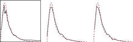
Fig. 12.2. Estimated probability density. Left hand: Nearest neighbor, center: Gaussian kernel, right hand: Polygon.

Some of the remedies for the di culties mentioned above use estimates of f and its derivatives. Thus iterative procedures seem to be the solution. However, the iteration process usually does not converge and thus has to be supervised and stopped before artifacts appear.

In Fig. 12.2 three simple smoothing methods are compared. A sample of 1000 events has been generated from the function shown as a dashed curve in the figure. A k-nearest neighbor approximation of the p.d.f. of a sample is shown in the left hand graph of Fig. 12.2. The value of k chosen was 100 which is too small to produce enough smoothing but too large to follow the distribution at the left hand border. The result of the PDE with a Gaussian kernel with fixed width is presented in the central graph and a polygon approximation is shown in the right-hand graph. All three graphs show the typical defects of simple smoothing methods, broadening of the peak and fake structures in the region where the statistics is low.

Alternatively to the standard smoothing methods, complementary approaches often produce better results than the former. The typical smoothing problems can partially be avoided when the p.d.f. is parameterized and adjusted to the data sample in a likelihood fit. A simple parametrization is the superposition of normal distributions, X

f(x) = αiN(x; µi, Σi) ,

with the free parameters, weights αi, mean values µi and covariance matrixes Σi.

If information about the shape of the distribution is available, more specific parameterizations which describe the asymptotic behavior can be applied. Distributions which resemble a Gaussian should be approximated by the Gram-Charlier series (see last paragraph of Sect. 11.2.2). If the data sample is su ciently large and the distribution is unimodal with known asymptotic behavior the construction of the p.d.f. from the moments as described in [74] is quite e cient.

Physicists use PDE mainly for the visualization of the data. Here, in one dimension, histogramming is the standard method. When the estimated distribution is used to simulate an experiment, frequency polygons are to be preferred. Whenever a useful parametrization is at hand, then PDE should be replaced by an adjustment of the corresponding parameters in a likelihood fit. Only in rare situations it pays to