Добавил:
Upload Опубликованный материал нарушает ваши авторские права? Сообщите нам.
Вуз: Предмет: Файл:

vstatmp_engl

.pdf
Скачиваний:
10
Добавлен:
12.03.2016
Размер:
6.43 Mб
Скачать


10.3 Goodness-of-Fit Tests 267

π0

(z)

≡ 1

,


π1

(z)

=


3(2z − 1) ,


. . . . . . . . .


πi(z) =


2i + 1Pi(2z − 1) .

Here Pi(x) is the Legendre polynomial in the usual form. The first parameter θ0 is fixed, θ0 = 1, and the other parameters are restricted such that gk is positive. The user has to choose the parameter k which limits the degree of the polynomials. If the alternative hypothesis is suspected to contain narrow structures, we have to admit large k. The test with k = 1 rejects a linear contribution, k = 2 in addition a quadratic component and so on. Obviously, the null hypothesis H0 corresponds to

θ1 = · · · = θk = 0, or equivalently to Pk θ2 = 0. We have to look for a test statistic

i=1 i

which increases with the value of this sum.

For a sample of size N the test statistic proposed by Neyman is


k


k

N


2


1

1


Xi


X

X


(10.9)

rk2 = N

=1

ti2 = N

i=1


πi(zj ) .


j=1


This choice is plausible, because a large absolute value of ti is due to a strong contribution of the polynomial πi to the observed distribution and thus also to a large value of θi2, while under H0 we have for i ≥ 1

htii = Nhπi(z)i = 0 ,

because

Z 1


πi(z) dz = 0 .


0

Asymptotically, N → ∞, under H0 the test statistic rk2 follows a χ2 distribution with k degrees of freedom (see 3.6.7). This is a consequence of the orthonormality of the polynomials πi and the central limit theorem: We have

var(ti) = hti2i = N Z0

1

πi2(z) dz = N

and as a sum of N random variables the statistic ti/ N is normally distributed for large N, with expectation value zero and variance one. Due to the orthogonality of the πi, the ti are uncorrelated. For small N the distribution of the test statistic rk2 has to be obtained by a Monte Carlo simulation.

In any case, large values of rk2 indicate bad agreement of the data with H0, but for a fixed value of k the smooth test is not consistent6. Its power approaches unity for N → ∞ only for the class of alternatives Hk having a PIT which is represented by an expansion in Legendre polynomials up to order k. Hence with respect to these, while usually uninteresting, restricted alternatives it is consistent. Thus for large samples and especially for the exclusion of narrow structures k should not be chosen too small. The value of k in the smooth test corresponds roughly to the number of bins in the χ2-test.

The smooth test is in most cases superior to the χ2 test. This can be understood in the following way: The smooth test scrutinizes not only for structures of a fixed

6For k = 1, for instance, the test cannot exclude distributions concentrated near z = 1/2.

268 10 Hypothesis Tests

frequency but for all frequencies up to k while the χ2 test with B 1 bins is rather insensitive to low frequency variations.

Remark: The alternative distribution quoted by Neyman was the exponential


Xi

θiπi(z)!


gk(z) = C exp

k

(10.10)


=0


where C(θ) is a normalization constant. Neyman probably chose the exponential form, because it guaranties positivity without further restrictions of the parameters θi. Moreover, with this class of alternatives, it has been shown by E. S. Pearson [60] that the smooth test can be interpreted as a likelihood ratio test. Anyway, (10.8) or (10.10) serve only as a motivation to choose the test statistic (10.9) which is the relevant quantity.

10.3.8 The L2 Test

The binning-free tests discussed so far are restricted to one dimension, i.e. to univariate distributions. We now turn to multivariate tests.

A very obvious way to express the di erence between two distributions f and f0 is the integrated quadratic di erence

Z

L2 = [f(r) − f0(r)]2 dr. (10.11)

Unfortunately, we cannot use this expression for the comparison of a sample {r1, . . . , rN } with a continuous function f0. Though we can try to derive from our sample an approximation of f. Such a procedure is called probability density estimation (PDE ).

A common approach (see Chap. 12) is the Gaussian smearing or smoothing. The N discrete observations at the locations ri are transformed into the function

fG(r) = N1 X eα(ri−r)2 .

The smearing produces a broadening which has also to be applied to f0:

Z

f0G(r) = f0(r)eα(r−r)2 dr.

We now obtain a useful test statistic L2G,

Z

L2G = [fG(r) − f0G(r)]2 dr .

So far the L2 test [61] has not found as much attention as it deserves because the calculation of the integral is tedious. However its Monte Carlo version is pretty simple. It o ers the possibility to adjust the width of the smearing function to the density f0. Where we expect large distances of observations, the Gaussian width should be large, α f02.

A more sophisticated version of the L2 test is presented in [61]. The Monte Carlo version is included in Sect. 10.3.11, see below.

10.3 Goodness-of-Fit Tests

269

10.3.9 Comparing a Data Sample to a Monte Carlo Sample and the Metric

We know turn to tests where we compare our sample not to an analytic distribution but to a Monte Carlo simulation of f0. This is not a serious restriction because anyhow acceptance and resolution e ects have to be taken into account in the majority of all experiments. Thus the null hypothesis is usually represented by a simulation sample.

To compare two samples we have to construct a relation between observations of the samples which in the multi-dimensional case has to depend in some way on the distance between them. We can define the distance in the usual way using the standard Euclidian metric but since the di erent dimensions often represent completely di erent physical quantities, e.g. spatial distance, time, mass etc., we have considerable freedom in the choice of the metric and we will try to adjust the metric such that the test is powerful.

We usually want that all coordinates enter with about equal weight into the test. If, for example, the distribution is very narrow in x but wide in y, then the distance r of points is almost independent of y and it is reasonable to stretch the distribution in the x direction before we apply a test. Therefore we propose for the general case to scale linearly all coordinates such that the empirical variances of the sample are the same in all dimensions. In addition we may want to get rid of correlations when for instance a distribution is concentrated in a narrow band along the x-y diagonal.

Instead of transforming the coordinates we can use the Mahalanobis distance7 in order to normalize distances between observations (x1, . . . , xN } with sample mean x. (The bold-face symbols here denote P -dimensional vectors describing di erent features measured on each of the N sampled objects.)

The Mahalanobis distance dM of two observations x and xis q

dM = (x − x)T C−1(x − x) ,

with

XN

Cij = (xni − xi)(xnj − xj )/N .

n=1

It is equivalent to the Euclidian distance after a linear transformation of the vector components which produces a sample with unity covariance matrix. If the covariance matrix is diagonal, then the resulting distance is the normalized Euclidean distance in the P -dimensional space:

dM = v


P

(xp 2xp)2 .

uX


t


up=1

σp

In the following tests the choice of the metric is up to the user. In many situations it is reasonable to use the Mahalanobis distance, even though moderate variations of the metric normally have little influence on the power of a test.

7This is a distance measure introduced by P. C. Mahalanobis in 1936.

270 10 Hypothesis Tests

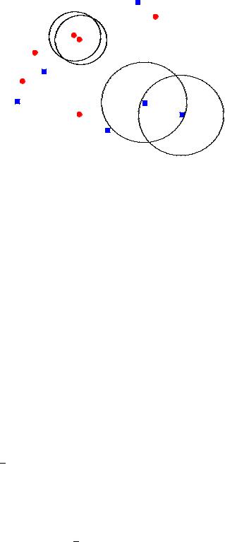
Fig. 10.11. K-nearest neighbor test.

10.3.10 The k-Nearest Neighbor Test

We consider two samples, one generated by a Monte Carlo simulation of a null distribution f0 and the experimental sample. The test statistic is the number n(k) of observations of the mixed sample where all of its k nearest neighbors belong to the same sample as the observation itself. This is illustrated in Fig. 10.11 for an unrealistically simple configuration. We find n(1) = 4 and n(2) = 4. The parameter k is a small number to be chosen by the user, in most cases it is one, two or three.

Of course we expect n to be large if the two parent distributions are very di erent. The k-nearest neighbor test is very popular and quite powerful. It has one caveat: We would like to have the number M of Monte Carlo observations much larger than the number N of experimental observations. In the situation with M N each observation tends to have as next neighbor a Monte Carlo observation and the test becomes less significant.

10.3.11 The Energy Test

A very general expression that measures the di erence between two distributions f(r) and f0(r) in an n dimensional space is

φ =

1

Z

dr Z

dr[f(r) − f0(r)] [f(r) − f0(r)] R(r, r) .

(10.12)

2

Here we call R the distance function. The factor 1/2 is introduced to simplify formulas which we derive later. The special case R = δ(r − r) leads to the simple integrated quadratic deviation (10.11) of the L2 test

φ =

1

Z

dr [f(r) − f0(r)]2 .

(10.13)

2

10.3 Goodness-of-Fit Tests

271

However, we do not intend to compare two distributions but rather two samples A {r1, . . . , rN }, B {r01, . . . , r0M }, which are extracted from the distributions f and f0, respectively. For this purpose we start with the more general expression (10.12) which connects points at di erent locations. We restrict the function R in such a way that it is a function of the distance |r − r| only and that φ is minimum for f ≡ f0.

The function (10.12) with R = 1/|r − r| describes the electrostatic energy of the sum of two charge densities f and f0 with equal total charge but di erent sign of the charge. In electrostatics the energy reaches a minimum if the charge is zero everywhere, i.e. the two charge densities are equal up to the sign. Because of this analogy we refer to φ as energy.
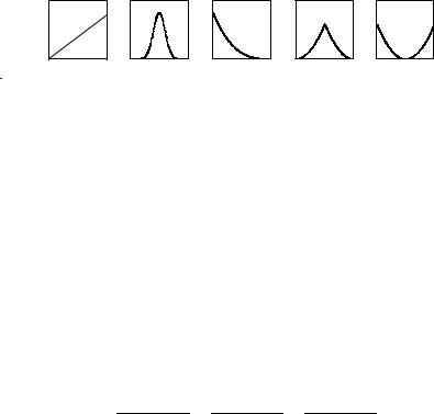
For our

purposes the logarithmic function R(r) =

ln(r) and the bell function


2

) are more suitable than 1/r.


R(r) exp(−cr


We multiply the expressions in brackets in (10.12) and obtain

1

Z

dr Z

dr[f(r)f(r) + f0(r)f0(r) − 2f(r)f0(r)] R(|r − r|) . (10.14)

φ =


2

A Monte Carlo integration of this expression is obtained when we generate M random

points {r01 . . . r0M } of the distribution f0(r) and N random points {r1, . . . , rN } of the distribution f(r) and weight each combination of points with the corresponding

distance function. The Monte Carlo approximation is:


X X


1

Xi

X


φ ≈


1


i j>i R(|ri rj |) −


R(|ri − r0j |) +

N(N


1)


NM


j


1


Xi

X


+


R(|r0i − r0j |)


M(M 1)


X X


j>i


Xi

X


1


1


R(|ri − rj |) −


R(|ri − r0j |) +


N2


i


j>i

NM


j


+

1


Xi

X

R(|r0i − r0j |) .


(10.15)


M2


j>i


This is the energy of a configuration of discrete charges. Alternatively we can understand this result as the sum of three expectation values which are estimated by the two samples. The value of φ from (10.15) thus is the estimate of the energy of two samples that are drawn from the distributions f0 and f and that have the total charge zero.

We can use the expression (10.15) as test statistic when we compare the experimental sample to a Monte Carlo sample, the null sample representing the null distribution f0. Small energies signify a good, large ones a bad agreement of the experimental sample with H0. To be independent of statistical fluctuations of the simulated sample, we choose M large compared to N, typically M ≈ 10N.

The test statistic energy φ is composed of three terms φ1, φ2, φ3 which correspond to the interaction of the experimental sample with itself, to its interaction with the null sample and with the interaction of the null sample with itself:

φ = φ1 − φ2 + φ3 ,

(10.16)


1


X

(10.17)

φ1 =

N(N


1)

i<j R(|ri rj|) ,

272 10 Hypothesis Tests


X


1

R(|ri − r0j |) ,

(10.18)

φ2

=


i,j

NM


1


X

(10.19)

φ3

=

M(M


1)

i<j R(|r0i r0j |) .

The term φ3 is independent of the data and can be omitted but is normally included to reduce statistical fluctuations.

The distance function R relates sample points and simulated points of the null hypothesis to each other. Proven useful have the functions

Rl = − ln(r + ε) ,

(10.20)

Rs = er2/(2s2) .

(10.21)

The small positive constant ε suppresses the pole of the logarithmic distance function. Its value should be chosen approximately equal to the experimental resolution8 but variations of ε by a large factor have no sizable influence on the result. With the function R1 = 1/r we get the special case of electrostatics. With the Gaussian distance function Rs the test is very similar to the χ2 test with bin width 2s but avoids the arbitrary binning of the latter. For slowly varying functions we propose to use the logarithmic distance function.

Empirical studies have shown that the test statistic follows to a very good approximation a distribution from the family of the extreme value distributions,


σ


σ


(


σ


)

f(φ) =

1


1 + ξ

φ − µ

−1−1 exp


1 + ξ

φ − µ

−1

,


with parameters µ, σ, ξ which we have discussed in Sect. 3.6.12. We have to compute this distribution f0(φ) by a Monte Carlo simulation. To get a su cient precision for small p-values we have to generate a very large sample. We gain computing time when we extract the first three moments of a relatively modest Monte Carlo sample and compute from those the parameters of the extreme value distribution.

The energy test is consistent [63]. It is quite powerful in many situations and has the advantage that it is not required to sort the sample elements.

The energy test with Gaussian distance function is completely equivalent to the L2 test. It is more general than the latter in that it allows to use various distance functions.

10.3.12 Tests Designed for Specific Problems

The power of tests depends on the alternatives. If we have an idea of it, even if it is crude, we can design a GOF test which is especially sensitive to the deviations from H0 which we have in mind. The distribution of the test statistic has to be produced by a Monte Carlo simulation.

Example 130. Designed test: three region test

8Distances between two points that are smaller than the resolution are accidental and thus insignificant.

10.3 Goodness-of-Fit Tests

273

A

B

C

Fig. 10.12. Di erent admixtures to a uniform distribution.

Experimental distributions often show a local excess of observations which are either just a statistical fluctuation or stem from a physical process. To check whether an experimental sample is compatible with the absence of a bump caused by a physical process, we propose the following three region test. We subdivide the domain of the variable in three regions with expected numbers of observations n10, n20, n30 and look for di erences to the corresponding experimental numbers n1, n2, n3. The subdivision is chosen such that the sum of the di erences is maximum. The test statistic R3 is

R3 = sup [(n1 − n10) + (n2 − n20) + (n3 − n30)] .

n1,n2

Notice, that n3 = N − n1 − n2 is a function of n1 and n2. The generalization to more than three regions is trivial. Like in the χ2 test we could also divide the individual squared di erences by their expected value:

R

= sup


(n1 − n10)2

+

(n2 − n20)2

+

(n3 − n30)2

.

3

n1,n2

n10


n20


n30


10.3.13 Comparison of Tests

Univariate Distributions

Whether a test is able to detect deviations from H0 depends on the distribution f0 and on the kind of distortion. Thus there is no test which is most powerful in all situations.

To get an idea of the power of di erent tests, we consider six di erent admixtures to a uniform distribution and compute the fraction of cases in which the distortion of the uniform distribution is detected at a significance level of 5%. For each distribution constructed in this way, we generate stochastically 1000 mixtures with 100 observations each. The distributions which we add are depicted in Fig. 10.12. One of them is linear, two are normal with di erent widths, and three are parabolic. The χ2 test was performed with 12 bins following the prescription of Ref. [58], the parameter of Neyman’s smooth test was k = 2 and the width of the Gaussian of the energy test was s = 1/8. The sensitivity of di erent tests is presented in Fig. 10.13.

The histogram of Fig. 10.13 shows that none of the tests is optimum in all cases. The χ2 test performs only mediocrely. Probably a lower bin number would improve the result. The tests of Neyman, Anderson–Darling and Kolmogorov–Smirnov are sensitive to a shift of the mean value while the Anderson–Darling test reacts especially to changes at the borders of the distribution. The tests of Watson and Kuiper detect preferentially variations of the variance. Neyman’s test and the energy test with logarithmic distance function are rather e cient in most cases.

274 10 Hypothesis Tests

power

1.0


0.5


0.0

30% B

20% N(0.5,1/24)

20% N(0.5,1/32)


power


Anderson


Kolmogorov


Kuiper


Neyman


1.0


Watson


Region


Energy(log)


Energy1(Gaussian)


Chi


0.5


0.0

50% linear

30% A

30% C


Fig. 10.13. Power (fraction of identified distortions) of di erent tests.

Multivariate Distributions

The goodness-of-fit of multivariate distributions cannot be tested very well with simple tests. The χ2 test often su ers from the small number of entries per bin. Here the k-nearest neighbor test and the energy test with the long range logarithmic distance function are much more e cient.

Example 131. GOF test of a two-dimensional sample

Figure 10.14 shows a comparison of a sample H1 with a two-dimensional normal distribution (H0). H1 corresponds to the distribution of H0 but contains an admixture of a linear distribution. The p-value of the energy test is 2%.

10.4 Two-Sample Tests

275

4

c2

)=0.71


p(


p(

)=0.02


F


2


0

-2


-4

-2

0

2


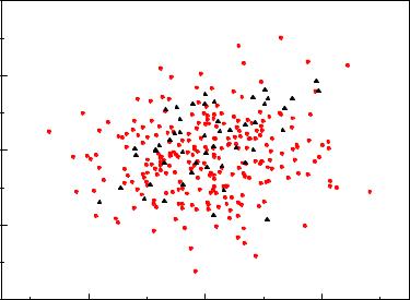
Fig. 10.14. Comparison of a normally distributed sample (circles) from H0 with a linear admixture (triangles) with the normal distribution of H0.

With a χ2 test with 9 bins we obtain a p-value of 71%. It is unable to identify the deformation of f0.

More detailed investigations can be found in [62].

10.4 Two-Sample Tests

10.4.1 The Problem

A standard situation in particle physics is that H0 cannot be compared directly to the data but has first to be transformed to a Monte Carlo sample, to take into account acceptance losses and resolution e ects. We have to compare two samples, a procedure which we had already applied in the energy test. Here the distribution of the test statistic needed to compute p-values can be generated by a simple Monte Carlo program.

In other sciences, a frequently occurring problem is that the e ectiveness of two or several procedures have to be compared. This may concern drugs, animal feed or the quality of fabrication methods. A similar problem is to test whether a certain process is stable or whether its results have changed during time. Also in the natural sciences we frequently come across the problem that we observe an interesting phenomenon in one data sample which apparently has disappeared in another sample taken at a later time. It is important to investigate whether the two data samples are compatible with each other. Sometimes it is also of interest to investigate whether a Monte Carlo sample and an experimental sample are compatible. Thus we are interested in

276 10 Hypothesis Tests

a statistical procedure which tells us whether two samples A and B are compatible, i.e. drawn from the same parent distribution. Thereby we assume that the parent distribution itself is unknown. If it were known, we could apply one of the GOF tests which we have discussed above. We have to invent procedures to generate the distribution of the test statistic. In some cases this is trivial. In the remaining cases, we have to use combinatorial methods.

10.4.2 The χ2 Test

To test whether two samples are compatible, we can apply the χ2test or the Kolmogorov–Smirnov test with minor modifications.

When we calculate the χ2 statistic we have to normalize the two samples A and B of sizes N and M to each other. For ai and bi entries in bin i, ai/N − bi/M should be compatible with zero. With the usual error propagation we obtain an estimate ai/N2 + bi/M2 of the quadratic error of this quantity and


Xi


χ2 =

B

(ai/N

− bi/M)2

.

(10.22)


=1

(ai/N2

+ bi/M2)


It follows approximately a a χ2 distribution of B − 1 degrees of freedom, but not exactly, as we had to replace the expected values by the observed numbers in the error estimation. We have to be careful if the number of observations per bin is small.

10.4.3 The Likelihood Ratio Test

The likelihood ratio test is less vulnerable to low event numbers than the χ2 test.

Setting r = M/N we compute the likelihood that we observe in a single bin a entries with expectation λ and b entries with expectation ρλ, where the hypothesis H0 is characterized by ρ = r:

L(λ, ρ|a, b) = eλλa eρλ(ρλ)b . a! b!

Leaving out constant factors the log-likelihood is

ln L = −λ(1 + ρ) + (a + b) ln λ + b ln ρ .

We determine the conditional maximum likelihood value of λ under ρ = r and the corresponding log-likelihood:

1 + r = (a + b)

1

,


ˆ


λc


ˆ

a + b


λc =


,


1 + r


+ b ln r .

ln Lcmax = (a + b) −1 + ln

a + b


1 + r

The unconditional maximum of the likelihood is found for ˆ and :

λ = a ρˆ = b/a

Соседние файлы в предмете [НЕСОРТИРОВАННОЕ]