vstatmp_engl

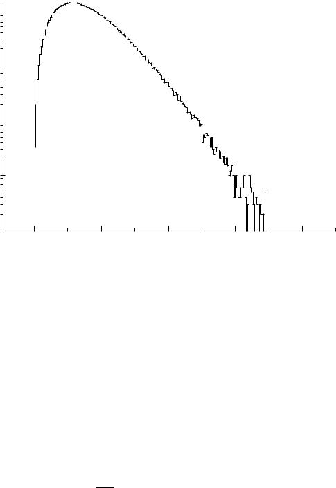
Fig. 5.6. Planck spectrum with majorant.

To generate

f(x) = c(e−0.2x sin2 x) for 0 < x < ∞

with the majorant

m(x) = c e−0.2x ,

we normalize m(x) and calculate its distribution function

Z x

r = 0.2e−0.2x′ dx′

0

= 1 − e−0.2x .

Thus the variate transformation from the uniformly distributed random number r1 to x is

1

x = − 0.2 ln(1 − r1) .

We draw a second uniform random number r2, also between zero and one, and test whether r2 m(x) exceeds the desired p.d.f. f(x). If this is the case, the event is rejected:

With this method a uniform distribution of random points below the majorant curve is generated, while only those points are kept which lie below the p.d.f. to be generated. On average about 4 random numbers per event are needed in this example, since the test has a positive result in about half of the cases.

If an appropriate continuous, analytical majorant function cannot be found, often a piecewise constant function (step function) is chosen.

118 5 Monte Carlo Simulation

10000

1000

y

100

10

1

Fig. 5.7. Generated Planck spectrum.

Example 65. Generation of the Planck distribution

Here a piecewise defined majorant is useful. We consider again the Planck distribution (5.1), and define the majorant in the following way: For small values x < x1 we chose a constant majorant m1(x) = 6 c. For larger values x > x1 the second majorant m2(x) should be integrable with invertible integral function. Due to the x3-term, the Planck distribution decreases somewhat more slowly than e−x. Therefore we chose for m2 an exponential factor with x substituted by x1−ε. With the arbitrary choice ε = 0.1 we take

m2(x) = 200 c x−0.1e−x0.9 .

The factor x−0.1 does not influence the asymptotic behavior significantly but permits the analytical integration:

Z x

M2(x) = m2(x′)dx′,

x1

=200c he−x01.9 − e−x0.9 i . 0.9

This function can be easily solved for x, therefore it is possible to generate m2 via a uniformly distributed random number. Omitting further details of the calculation, we show in Fig. 5.6 the Planck distribution with the two majorant pieces in logarithmic scale, and in Fig. 5.7 the generated spectrum.

5.2.5 Treatment of Additive Probability Densities

Quite often the p.d.f. to be considered is a sum of several terms. Let us restrict ourselves to the simplest case with two terms,

f(x) = f1(x) + f2(x) ,

with

Z ∞

S1 = f1(x)dx ,

Z−∞∞

S2 = f2(x)dx ,

−∞

S1 + S2 = 1 .

Now we chose with probability S1 (S2) a random number distributed according to f1 (f2). If the integral functions

Z x

F1(x) = f1(x′)dx′ ,

Z−x∞

F2(x) = f2(x′)dx′

−∞

are invertible, we obtain with a uniformly distributed random number r the variate x distributed according to f(x):

x = F1−1(r) for r < S1 ,

respectively

x = F2−1(r − S1) for r > S1 .

The generalization to more than two terms is trivial.

Example 66. Generation of an exponential distribution with constant background

and for r > ε

r − ε x = a 1 − ε .

We need only one random number per event. The direct way to use the inverse of the distribution function F (x) would not have been successful, since it cannot be given in analytic form.

The separation into additive terms is always recommended, even when the individual terms cannot be handled by simple variate transformations as in the example above.

120 5 Monte Carlo Simulation

5.2.6 Weighting Events

In Sect. 3.6.3 we have discussed some statistical properties of weighted events and

realized that the relative statistical error of a sum of N weighted events can be much

√

larger than the Poisson value 1/ N, especially when the individual weights are very di erent. Thus we will usually refrain from weighting. However, there are situations where it is not only convenient but essential to work with weighted events. If a large sample of events has already been generated and stored and the p.d.f. has to be changed afterwards, it is of course much more economical to re-weight the stored events than to generate new ones because the simulation of high energy reactions in highly complex detectors is quite expensive. Furthermore, for small changes the weights are close to one and will not much increase the errors. As we will see later, parameter inference based on a comparison of data with a Monte Carlo simulation usually requires re-weighting anyway.

An event with weight w stands for w identical events with weight 1. When interpreting the results of a simulation, i.e. calculating errors, one has to take into account the distribution of a sum of weights, see last example in Sect. 4.3.6. There we showed that X X

var wi = wi2 . Relevant is the relative error of a sum of weights:

Strongly varying weights lead to large statistical fluctuations and should therefore be avoided.

To simulate a distribution

f(x) : with xa < x < xb

with weighted events is especially simple: We generate events xi that are uniformly distributed in the interval [xa, xb] and weight each event with wi = f(xi).

In the Example 64 we could have generated events following the majorant distribution, weighting them with sin2 x. The weights would then be wi = f(xi)/m(xi).

When we have generated events following a p.d.f. f(x|θ) depending on a parameter θ and are interested in the distribution f′(x|θ′) we have only to re-weight the events by f′/f.

5.2.7 Markov Chain Monte Carlo

Introduction

The generation of distributions of high dimensional distributions is di cult with the methods that we have described above. Markov chain Monte Carlo (MCMC) is able to generate samples of distributions with hundred or thousand dimensions. It has become popular in thermodynamics where statistical distributions are simulated to compute macroscopic mean values and especially to study phase transitions. It has also been applied for the approximation of functions on discrete lattices. The method

is used mainly in theoretical physics to sample multi-dimensional distributions, sofar we know of no applications in experimental particle physics. However, MCMC is used in artificial neural networks to optimize the weights of perceptron nets.

Characteristic of a Markov chain is that a random variable x is modified stochastically in discrete steps, its value at step i depending only on its value at the previous

step i − 1. Values of older steps are forgotten: P (xi|xi−1, xi−2, ..., x1) = P (xi|xi−1). A typical example of a Markov chain is random walk. Of interest are Markov chains

that converge to an equilibrium distribution, like random walk in a fixed volume. MCMC generates a Markov chain that has as its equilibrium distribution the desired distribution. Continuing with the chain once the equilibrium has been reached produces further variates of the distribution. To satisfy this requirement, the chain has to satisfy certain conditions which are fulfilled for instance for the so-called Metropolis algorithm, which we will use below. There exist also several other sampling methods. Here we will only sketch this subject and refer the interested reader to the extensive literature which is nicely summarized in [27].

Thermodynamical Model, Metropolis Algorithm

In thermodynamics the molecules of an arbitrary initial state always approach – if there is no external intervention – a stationary equilibrium distribution. Transitions then obey the principle of detailed balance. In a simple model with atoms or molecules in only two possible states in the stationary case, the rate of transitions from state 1 to state 2 has to be equal to the reverse rate from 2 to 1. For occupation numbers N1, N2 of the respective states and transition rates per molecule and time W12, respectively W21, we have the equation of balance

N1W12 = N2W21 .

For instance, for atoms with an excited state, where the occupation numbers are very di erent, the equilibrium corresponds to a Boltzmann distribution, N1/N2 = e−ΔE/kT , with ΔE being the excitation energy, k the Boltzmann constant and T the absolute temperature. When the stationary state is not yet reached, e.g. the number N1 is smaller than in the equilibrium, there will be less transitions to state 2 and more to state 1 on average than in equilibrium. The occupation number of state 1 will therefore increase until equilibrium is reached. Since transitions are performed stochastically, even in equilibrium the occupation numbers will fluctuate around their nominal values.

If now, instead of discrete states, we consider systems that are characterized by a continuous variable x, the occupation numbers are to be replaced by a density distribution f(x) where x is multidimensional. It represents the total of all energies of all molecules. As above, for a stationary system we have

f(x)W (x → x′) = f(x′)W (x′ → x) .

As probability P (x → x′) for a transition from state x to a state x′ we choose the Boltzmann acceptance function

122 5 Monte Carlo Simulation

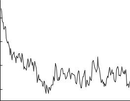
Fig. 5.8. Mean distance of spheres as a function of the number of iterations.

In an ideal gas and in many other systems the transition regards only one or two molecules and we need only consider the e ect of the change of those. Then the evaluation of the transition probability is rather simple. Now we simulate the stochastic changes of the states with the computer, by choosing a molecule at random and change its state with the probability P (x → x′) into a also randomly chosen state x′ (x → x′). The choice of the initial distribution for x is relevant for the speed of convergence but not for the asymptotic result.

This mechanism has been introduced by Metropolis et al. [28] with a di erent acceptance function in 1953. It is well suited for the calculation of mean values and fluctuations of parameters of thermodynamical or quantum statistical distributions. The process continues after the equilibrium is reached and the desired quantity is computed periodically. This process simulates a periodic measurement, for instance of the energy of a gas with small number of molecules in a heat bath. Measurements performed shortly one after the other will be correlated. The same is true for sequentially probed quantities of the MCMC sampling. For the calculation of statistical fluctuations the e ect of correlations has to be taken into account. It can be estimated by varying the number if moves between subsequent measurements.

Example 67. Mean distance of gas molecules

We consider an atomic gas enclosed in a cubic box located in the gravitational field of the earth. The N atoms are treated as hard balls with given radius R. Initially the atoms are arranged on a regular lattice. The p.d.f. is zero for overlapping atoms, and proportional to e−αz, where z is the vertical coordinate of a given atom. The exponential factor corresponds to the Boltzmann distribution for the potential energy in the gravitational field. An atom is chosen randomly. Its position may be (x, y, z). A second position inside the box is randomly selected by means of three uniformly distributed random numbers. If within a distance of less than 2R an other atom is found, the move is rejected and we repeat the selection of a possible new location. If the position search with the coordinates (x′, y′, z′) is successful, we form the ratio

z

x

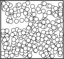
Fig. 5.9. Solid sheres in a box. The plot is a projection onto the x-z plane.

w = e−az′ /(e−az′ + e−αz). The position is changed if the condition r < w is fulfilled, with a further random number r. Periodically, the quantity being studied, here the mean distance between atoms, is calculated. It is displayed in Fig. 5.8 as a function of the iteration number. Its mean value converges to an asymptotic value after a number of moves which is large compared to the number of atoms. Fig. 5.9 shows the position of atoms projected to the x-z plane, for 300 out of 1000 considered atoms, after 20000 moves. Also

the statistical fluctuations can be found and, eventually, re-calculated for a

√

modified number of atoms according to the 1/ N-factor.

5.3 Solution of Integrals

The generation of distributions has always the aim, finally, to evaluate integrals. There the integration consists in simply counting the sample elements (the events), for instance, when we determine the acceptance or e ciency of a detector.

The integration methods follow very closely those treated above for the generation of distributions. To simplify the discussion, we will consider mainly one-dimensional integrals. The generalization to higher dimensions, where the advantages of the Monte Carlo method become even more pronounced than for one-dimensional integration, does not impose di culties.

Monte Carlo integration is especially simple and has the additional advantage that the accuracy of the integrals can be determined by the usual methods of statistical error estimation. Error estimation is often quite involved with the conventional numerical integration methods.

5.3.1 Simple Random Selection Method

Integrals with the integrand changing sign are subdivided into integrals over intervals with only positive or only negative integrand. Hence it is su cient to consider only

124 5 Monte Carlo Simulation

As in the analogous case when we generate a distribution, we produce points which are distributed randomly and uniformly in a rectangle covering the integrand function. An estimate I for the area I is obtained from the ratio of successes – this are the points falling below the function y(x) – to the number of trials N0, multiplied

To evaluate the uncertainty of this estimate, we refer to the binomial distribution in which we approximate the probability of success ε by the experimental value

ε = N/N0:

As expected, the accuracy raises with the square root of the number of successes and with ε. The smaller the deviation of the curve from the rectangle, the less will be the uncertainty.

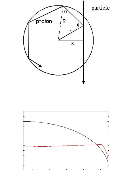
Example 68. Photon-yield for a particle crossing a scintillating fiber

Ionizing particles are crossing a scintillating fiber with circular cross section perpendicular to the fiber axis which is parallel to the z-axis (Fig. 5.10), and generate photons with spatially isotropic angular distribution (see 5.2.2). Photons hitting the fiber surface will be reflected if the angle with respect to the surface normal is larger than β0 = 60o. For smaller angles they will be lost. We want to know, how the number of captured photons depends on the location where the particle intersects the fiber. The particle traverses the fiber in y direction at a distance x from the fiber axis. To evaluate the acceptance, we perform the following steps:

• Set the fiber radius R = 1, create a photon at x, y uniformly distributed in the square 0 < x , y < 1,

•calculate r2 = x2 + y2, if r2 > 1 reject the event,

•chose azimuth angle ϕ for the photon direction, with respect to an axis parallel to the fiber direction in the point x, y, 0 < ϕ < 2π, ϕ uniformly distributed,

•calculate the projected angle α (sin α = r sin ϕ),

•choose a polar angle ϑ for the photon direction, 0 < cos(ϑ) < 1, cos(ϑ) uniformly distributed,

•calculate the angle β of the photon with respect to the (inner) surface normal of the fiber, cos β = sin ϑ cos α,

•for β < β0 reject the event,

•store x for the successful trials in a histogram and normalize to the total number of trials.

Fig. 5.10. Geometry of photon radiation in a scintillating fiber.

track position

Fig. 5.11. Photon yield as a function of track position.

The e ciency is normalized such that particles crossing the fiber at x = 0 produce exactly 1 photon. Fig. 5.11 shows the result of our simulation. For large values of x the track length is small, but the photon capture e ciency is large, therefore the yield increases with x almost until the fiber edge.

126 5 Monte Carlo Simulation

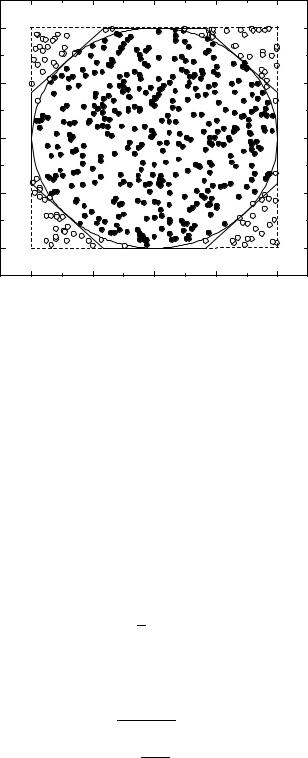
Fig. 5.12. Estimation of the number π.

5.3.2 Improved Selection Method

a) Reducing the Reference Area

We can gain in accuracy by reducing the area in which the points are distributed, as above by introduction of a majorant function, Fig. 5.5. As seen from (5.3), the relative error is proportional to the square root of the ine ciency.

We come back to the first example of this chapter:

Example 69. Determination of π

The area of a circle with radius 1 is π. For N0 uniformly distributed trials in a circumscribed square of area 4 (Fig. 5.12) the number of successes N is on average

An estimate πb for π is

Choosing a circumscribed octagon as the reference area, the error is reduced by about a factor two. A further improvement is possible by inscribing an-