vstatmp_engl

Добавил:

Upload Опубликованный материал нарушает ваши авторские права? Сообщите нам.

Вуз:

Южный Федеральный Университет

Предмет:

[НЕСОРТИРОВАННОЕ]

Файл:

sub-volume of 1 µm3

is then λ = 10 and its standard deviation for a Poisson

≈ 3. The exact calculation of the standard deviation

distribution is σ =

≈ 3. The exact calculation of the standard deviation

with the binomial distribution would change σ only by a factor

.pdf

Скачиваний:

Добавлен:

12.03.2016

Размер:

6.43 Mб

Скачать

☆

<<< < Предыдущая 1 2 3 4 5 6 78 / 428 9 10 11 12 13 14 15 16 17 18 19 20 21 22 23 24 25 > Следующая >>>

3.6 Some Important Distributions

There is no particularly simple expression for higher moments; they can of course be calculated from the Taylor expansion of φ(t), as explained in Sect. 3.3.2. We give only the results for the coe cients of skewness and excess:

γ		=		1 − 2p		, γ		=	1 − 6p(1 − p)	.
	1		pnp(1 − p)				2		np(1 − p)

Example 36. E ciency ﬂuctuations of a Geiger counter

A Geiger counter with a registration probability of 90% (p = 0.9) detects n′ out of n = 1000 particles crossing it. On average this will be hn′i =

np = 900. The mean ﬂuctuation (standard deviation) of this number is σ =
p			√
	np(1 − p) =		90 ≈ 9.5. The observed e ciency ε = n′/n will ﬂuctuate by
		p	p(1	−	p)/n	≈	0.0095
σε = σ/n =

Example 37. Accuracy of a Monte Carlo integration

We want to estimate the value of π by a Monte Carlo integration. We distribute randomly n points in a square of area 4 cm2, centered at the origin. The number of points with a distance less than 1 cm from the origin is k = np with p = π/4. To reach an accuracy of 1% requires

npσ = 0.01 ,

np(1 − p) = 0.01 , np

n =	(1 − p)	=	(4 − π)	≈	2732 ,
	0.012p		0.012π

i.e. we have to generate n = 2732 pairs of random numbers.

Example 38. Acceptance ﬂuctuations for weighted events

The acceptance of a complex detector is determined by Monte Carlo simulation which depends on a probability density f0(x) where x denotes all relevant kinematical variables. In order to avoid the repetition of the simulation for a di erent physical situation (e.g. a di erent cross section) described by a p.d.f. f(x), it is customary to weight the individual events with wi = f(x)/f0(x), i = 1, . . . , N for N generated events. The acceptance εi for event i is either 1 or 0. Hence the overall acceptance is

εT = Pwiεi . wi

The variance for each single term in the numerator is wi2εi(1 − εi). Then the variance σT2 of εT becomes

	P	w2	εi(1 εi)
σT2 =	P	(i	wi)−2	.
		P

58 3 Probability Distributions and their Properties

3.6.2 The Multinomial Distribution

When a single experiment or trial has not only two, but N possible outcomes with probabilities p1, p2, . . . , pN , the probability to observe in n experiments k1, k2, . . . , kN trials belonging to the outcomes 1, . . . , N is equal to

								n!		N
		Mn				(k , k , . . . , k ) =		n!		pki	,

					N			Q
		N			N	1 2	N	Q		iY
		p1	,p2,...,pN			1 2	N	N	ki!	i
	P			P				i=1		=1
where	P	i=1 pi = 1 and		P	i=1 ki = n are satisﬁed. Hence we have N − 1 independent
variates. The value N = 2 reproduces the binomial distribution.

In complete analogy to the binomial distribution, the multinomial distribution may be generated by expanding the multinom

(p1 + p2 + . . . + pN )n = 1

in powers of pi, see (3.43). The binomial coe cients are replaced by multinomial coe cients which count the number of ways in which n distinguishable objects can be distributed into N classes which contain k1, . . . , kN objects.

The expected values are

E(ki) = npi and the covariance matrix is given by

Cij = npi(δij − pj ) .

They can be derived from the characteristic function

	N−1		!	n
	N−1
	X
φ(t1, . . . , tN−1) = 1 +	1	pi eiti − 1

which is a straight forward generalization of the 1-dimensional case (3.44). The correlations are negative: If, for instance, more events ki as expected fall into class i, the mean number of kj for any other class will tend to be smaller than its expected value E(kj ).

The multinomial distribution applies for the distribution of events into histogram bins. For total a number n of events with the probability pi to collect an event in bin i, the expected number of events in that bin will be ni = npi and the variance Cii = npi(1 − pi). Normally a histogram has many bins and pi 1 for all i. Then we approximate Cij ≈ niδij . The correlation between the bin entries can be neglected and the ﬂuctuation of the entries in a bin is described by the Poisson distribution which we will discuss in the following section.

3.6.3 The Poisson Distribution

When a certain reaction happens randomly in time with an average frequency λ in a given time interval, then the number k of reactions in that time interval will follow a Poisson distribution (Fig. 3.15)

Pλ(k) = e−λ λk . k!

									3.6	Some Important Distributions							59
0.4									0.20
0.4									0.20
P						l	= 1		P						l	= 5


0.3									0.15
0.3									0.15
0.2									0.10


0.1									0.05




0.0									0.00



	0	2	4	6			8	10		0	5	10	15				20
					k							k
P
									P
									P
0.08						l	= 20		0.04					l		= 100
0.08						l	= 20		0.04					l		= 100
0.06




0.04									0.02




0.02




0.00									0.00

	0		20				40					100					150
	0		20				40					100					150
					k							k

Fig. 3.15. Poisson distributions with di erent expected values.

60 3 Probability Distributions and their Properties

Its expected value and variance have already been calculated above (see p. 36):

E(k) = λ , var(k) = λ .

The characteristic function and cumulants have also been derived in Sect. 3.3.2 :

φ(t) = exp λ(eit − 1) , (3.45)

κi = λ , i = 1, 2, . . . .

Skewness and excess,

1				1
γ1 =	√		, γ2 =
				λ
		λ

indicate that the distribution becomes more Gaussian-like with increasing λ (see Fig. 3.15).

The Poisson distribution itself can be considered as the limiting case of a binomial distribution with np = λ, where n approaches inﬁnity (n → ∞) and, at the same time, p approaches zero, p → 0. The corresponding limit of the characteristic function of the binomial distribution (3.44) produces the characteristic function of the Poisson distribution (3.45): With p = λ/n we then obtain

		λ					n
lim			(e	it		1)	= exp		it

	1 + n				−			λ(e		− 1) .
n→∞

For the Poisson distribution, the supply of potential events or number of trials is supposed to be inﬁnite while the chance of a success, p, tends to zero. It is often used in cases where in principle the binomial distribution applies, but where the number of trials is very large.

Example 39. Poisson limit of the binomial distribution

A volume of 1 l contains 1016 hydrogen ions. The mean number of ions in a

Also the number of radioactive decays in a given time interval follows a Poisson distribution, if the number of nuclei is big and the decay probability for a single nucleus is small.

The Poisson distribution is of exceptional importance in nuclear and particle physics, but also in the ﬁelds of microelectronics (noise), optics, and gas discharges it describes the statistical ﬂuctuations.

Speciﬁc Properties of the Poisson Distribution

The sum k = k1 + k2 of Poisson distributed numbers k1, k2 with expected values λ1, λ2 is again a Poisson distributed number with expected value λ = λ1 + λ2. This property, which we called stability in connection with the binomial distribution follows formally from the structure of the characteristic function, or from the additivity of the cumulants given above. It is also intuitively obvious.

	3.6 Some Important Distributions	61
Example 40. Fluctuation of a counting rate minus background
Expected are S signal events with a mean background B. The mean ﬂuctu-
ation (standard deviation) of the observed number k is √S + B. This is also
the ﬂuctuation of k − B, because B is a constant. For a mean signal S = 100
and an expected background B = 50 we will observe on average 150 events
with a ﬂuctuation of	√
	150. After subtracting the background, this ﬂuctua-

tion will remain. Hence, the background corrected signal is expected to be

√

100 with the standard deviation σ = 150. The uncertainty would even be larger, if also the mean value B was not known exactly.

If from a Poisson-distributed number n with expected value λ0 on the average only a fraction ε is registered, for instance when the size of a detector is reduced by a factor of ε, then the expected rate is λ = λ0ε and the number of observed events k follows the Poisson distribution Pλ(k). This intuitive result is also obtained analytically: The number k follows a binomial distribution Bεn(k) where n is a Poisson-distributed number. The probability p(k) is:

X∞

p(k) = Bn(k)P				(n)
	ε		λ0
n=k
∞		n!								λn
X		−		εk(1		−	ε)n−ke−λ0			0
=				εk(1			ε)n−ke−λ0
n=k k!(n k)!										n!
	(ελ0)k		∞			1
			X						− λ0ε)n−k
= e−λ0		k!	X		(n	−	k)!	(λ0	− λ0ε)n−k
			n=k

=e−ελ0 (ελ0)k k!

=Pλ(k) .

Of interest is also the following mathematical identity

k			Zλ∞ dλ′Pλ′ (k) ,
X
i=0 Pλ(i) =
k λi			∞ λ )k ′
X			Zλ	( ′
i=0	i!	e−λ =		k!	e−λ dλ′ ,

which allows us to calculate the probability P {i ≤ k} to ﬁnd a number i less or equal k via a well known integral (described by the incomplete gamma function). It is applied in the estimation of upper and lower interval limits in Chap. 8.

Weighted Poisson Distributed Events

Let us assume that we measure the activity of a β-source with a Geiger counter. The probability that it ﬁres, the detection probability, depends on the electron energy which varies from event to event. We can estimate the true number of decays by weighting each observation with the inverse of its detection probability. The statistics of their weighted sum is rather complex.

The statistics of weighted events plays also a role in some Monte Carlo integration methods, and sometimes also in parameter inference, if weighted observations

62 3 Probability Distributions and their Properties

	0.2				< k > = 4.8
					< k > = 4.8
probability	0.1
probability
	0.0	0	5	10	k	15	20
	0.10				k
	0.10				< k > = 24
					< k > = 24
probability	0.05
probability
	0.00	0	10	20	30	40	50
				k

Fig. 3.16. Comparison of Poisson distributions (histograms) and scaled distribution of weighted events (dots) with a mixture of weights of one and ten.

are given in the form of histograms. The probability distribution of the corrected numbers does not have a simple analytical expression. It can, as we will see, be approximately described by a Poisson distribution. However, the cumulants and thus also the moments of the distribution can be calculated exactly.

Let us consider the deﬁnite case that on average λ1 observations are obtained with probability ε1 and λ2 observations with probability ε2. We correct the losses by weighting the observed numbers with w1 = 1/ε1 and w2 = 1/ε2. For the Poissondistributed numbers k1, k2

3.6 Some Important Distributions

λk1 −λ

Pλ1 (k1) = k1 ! e 1 ,

λk2 −λ

Pλ2 (k2) = k2 ! e 2 ,

k = w1k1 + w2k2 ,

we get the mean value λ of the variate k and its variance with var(cx) = c2var(x):

λ = w1λ1 + w2λ2 ,

σ2 = w12λ1 + w22λ2 .

According to (3.28), the cumulant κi of order i of the distribution of k is related to the cumulants κ(1)i , κ(2)i of the corresponding distributions of k1, k2 through

κi = wi	κ(1)	+ wi	κ(2) .	(3.46)
1	i	2	i

As mentioned above, there is no simple closed expression for the distribution of k. It can be constructed approximately using the lower moments, but this is rather tedious. Therefore we try to describe it approximately by a scaled Poisson distribution

		˜
	˜k		˜
P˜ (k˜) =	λ		˜
			e−λ ,
	˜		e−λ ,
λ	˜
	k!

such that the ratio of standard deviation to mean value is the same as for the weighted sum. We obtain

	˜		σ
	λ	=	σ	,
˜		=	λ	,
λ
p			(w1λ1 + w2λ2)2
	˜		(w1λ1 + w2λ2)2					,
	λ =
	λ =			w2	λ1	+ w2	λ2
				1		2

where we have to scale the random variable ˜ to obtain the acceptance corrected k

number k:

˜	λ
k = k	˜
	λ
˜	w2	λ + w2		λ
˜	1	1	2	2

= k w1λ1 + w2λ2 .

The approximate distribution of k that we have obtained in this way has by construction the right mean value and width, but di ers from the exact distribution

in details. The quantity ˜ is called . A number of k equivalent number of events k

observations which has been corrected for acceptance losses has the same statistical

signiﬁcance as ˜ un-weighted observations. (The statistical signiﬁcance is the ratio of k

mean value to standard deviation µ/σ). The accuracy of our approximation can be checked by comparing the skewness and excess γ1,2 as obtained from the cumulants

(3.46) according to (3.27) with the results of a Poisson distribution, namely γ˜1 = p

˜ ˜.

1/ λ , γ2 = 1/λ

Example 41. Distribution of weighted, Poisson distributed observations

We expect on average λ1 = 20 observations registered with the probability ε1 = 0.1 (w1 = 10), and λ2 = λ1 = 20 observations with acceptance

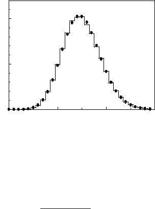
64 3 Probability Distributions and their Properties

probability

0.10	< k > = 15

0.05

0.000

Fig. 3.17. Comparison of a Poisson distribution (histogram) with a scaled distribution of weighted events (dots). The weights are uniformly distributed between zero and one.

ε1 = 1. The expected value of the acceptance corrected number is λ = 220. We approximate the distribution of the observed numbers k by the Poisson

distribution with the mean value ˜,

λ˜ =	(10 · 20 + 1 · 20)2	= 24.0 ,
	102 · 20 + 12 · 20

in order to describe the distribution of ˜. The statistical signiﬁcance of the

k 40 expected observations is the same as that of 24 unweighted observations. We


		˜ ˜ ˜	· 220/24 by generating
obtain the approximate distribution of k = kλ/λ = k			· 220/24 by generating
the distribution of	˜	and equating the probabilities of k and		˜
the distribution of	k	and equating the probabilities of k and		k. Fig. 3.16

shows a comparison between the equivalent Poisson distribution and the

true distribution of ˜ . By construction, mean value and variance are the kλ/λ

same; also skewness and excess are similar in both cases: The approximate (exact) values are, respectively, γ1 = 0.204 (0.221), γ2 = 0.042 (0.049). The di erences are partially due to the fact that we compare two di erent discrete distributions which have discrete parameters γ1, γ2.

The generalization of the above procedure to the addition of more than two weighted Poisson distributions is trivial:

˜	(		wiλi)2
λ =				,

k ≈ k		P wi2λi
			P wiλi .
	˜ P wi2λi
			P

For the sum of N accidental weights which follow a continuous distribution g(w),
we obtain the expected value λ = hki = N R g(w)w2dw and with λi = 1
˜	R	d
		g(w)w dw
λ = N	R	g(w)w2 w ,

		3.6 Some Important Distributions	65
k ≈ k˜	R	w)w2 dw
		gg((w)w dw .
	R

In Fig. 3.17, a scaled distribution with uniformly distributed weights between zero and one is compared to the corresponding approximating Poisson distribution. The agreement is quite good.

3.6.4 The Uniform Distribution

The uniform distribution is the simplest continuous distribution. It describes, for instance, digital measurements where the random variable is tied to a given interval and where inside the interval all its values are equally probable.

Given an interval of length α centered at the mean value ξ the p.d.f. reads

f(x ξ, α) =		1/α if \|x − ξ\| < α/2	(3.47)
\|		0 else .

Mean value and variance are hxi = ξ and σ2 = α2/12, respectively. The characteristic function is

	1	ξ+α/2		2		αt
φ(t) =		Zξ−α/2	eitxdx =		sin		eiξt .	(3.48)

	α			αt		2

Using the power expansion of the sinus function we ﬁnd from (3.48) for ξ = 0 the even moments (the odd moments vanish):

	1	α	2k
µ2′ k =			, µ2′ k−1 = 0 .
	2k + 1	2

The uniform distribution is the basis for the computer simulation of all other distributions because random number generators for numbers uniformly distributed between 0 and 1 are implemented on all computers used for scientiﬁc purposes. We will discuss simulations in some detail in Chap. 5.

3.6.5 The Normal Distribution

The normal or Gauss distribution which we introduced already in Sect. 3.2.7,

enjoys great popularity among statisticians. This has several reasons which, however, are not independent from each other.

1. The sum of normally distributed quantities is again normally distributed (sta-

P P

bility), with µ = µi, σ2 = σi2, in obvious notation.

2.The discrete binomialand Poisson distributions and also the χ2-distribution, in the limit of a large number, a large mean value and many degrees of freedom, respectively, approach the normal distribution.

3.Many distributions met in natural sciences are well approximated by normal distributions. We have already mentioned some examples: velocity components of gas

66 3 Probability Distributions and their Properties

molecules, di usion, Brownian motion and many measurement errors obey normal distributions to good accuracy.

4. Certain analytically simple statistical procedures for parameter estimation and propagation of errors are valid exactly only for normally distributed errors.

The deeper reason for point 2 and 3 is explained by the central limit theorem: The mean value of a large number N of independent random variables, obeying the same distribution with variance σ02, approaches a normal distribution with variance σ2 = σ02/N. The important point is that this theorem is valid for quite arbitrary distributions, provided they have a ﬁnite variance, a condition which practically always can be fulﬁlled, if necessary by cutting o large absolute values of the variates. Instead of a formal proof12, we show in Fig. 3.18, how with increasing number of variates the distribution of their mean value approaches the normal distribution better and better.

As example we have chosen the mean values for uniformly resp. exponentially distributed numbers. For the very asymmetrical exponential distribution on the left hand side of the ﬁgure the convergence to a normal distribution is not as fast as for the uniform distribution, where already the distribution of the mean of ﬁve random numbers is in good agreement with the normal distribution. The central limit theorem applies also when the individual variates follow di erent distributions provided that the variances are of the same order of magnitude.

The characteristic function of the normal distribution is

φ(t) = exp(− 12 σ2t2 + iµt) .

It is real and also of Gaussian shape for µ = 0. The stability (see point 1 above) is easily proven, using the convolution theorem (3.25) and the exponential form of φ(t).

Di erentiating the characteristic function, setting µ = 0, we obtain the central moments of the normal distribution:

µ′ = (2j)! σ2j .

2j 2jj!

Cumulants, with the exception of κ1 = µ and κ2 = σ2, vanish. Also the odd central moments are zero.

The Normal Distribution in Higher Dimensions

The normal distribution in two dimensions with its maximum at the origin has the general form

N0	(x, y) = p1 − ρ2	2πsxsy	exp	− 2(1 − ρ2)	sx2	− 2ρ sxsy	+ sy2		. (3.49)
	1			1	x2	xy	y2

The notation has been chosen such that it indicates the moments:

x2	= sx2	,

y2	= sy2	,

hxyi = ρsxsy .

12A simpliﬁed proof is presented in the Appendix 13.1.

<<< < Предыдущая 1 2 3 4 5 6 78 / 428 9 10 11 12 13 14 15 16 17 18 19 20 21 22 23 24 25 > Следующая >>>

Соседние файлы в предмете [НЕСОРТИРОВАННОЕ]

#
13.02.201531.06 Кб27Voprosy_lichnost_v_prof_deyatelnosti.docx
#
20.09.2019556.03 Кб7Voprosy_po_distsipline2 - копия.doc
#
27.09.2019275.97 Кб18voprosy_po_spets_kursu_k_zachetu.doc
#
23.09.2019653.82 Кб83Voprosy_vnimanie_i_pamyat_1.doc
#
02.08.201928.44 Кб8Vopros_10.docx
#
12.03.20166.43 Mб9vstatmp_engl.pdf
#
13.02.20151.12 Mб13Vsya_teoria_k_FAYa.pdf
#
14.11.2019212.99 Кб8Vvedenie_v_ specialnoct_kl.doc
#
11.11.2019739.33 Кб8vvedenie_v_socialno_ekonomicheskuyu_geografiyu.doc
#
08.11.201963.49 Кб1vvodnyy_urok_10_kl.doc
#
12.03.20161.99 Mб13web.doc