Biomolecular Sensing Processing and Analysis - Rashid Bashir and Steve Wereley

deriving a CM factor very similar to Eqn (8.2) but with an effective complex permittivity ε p that subsumes the effects of the complicated interior (see §5.3 of Hughes [39]). This process can be repeated multiple times to model general multi-shelled particles.

Membrane-Covered Spheres: Mammalian Cells, Protoplasts Adding a thin shell to a uniform sphere makes a decent electrical model for mammalian cells and protoplasts. The thin membrane represents the insulating cell membrane while the sphere represents the cytoplasm. The nucleus is not modeled is this approximation. For this model the effective complex permittivity can be represented by:

where εcyt o is the complex permittivity of the cytoplasmic compartment and cm refers to complex membrane capacitance per unit area and is given by

where cm and gm are the membrane capacitance and conductance per unit area (F/m2 and S/m2) and can be related to the membrane permittivity and conductivity by cm = εm /t and gm = σm /t , where t is the membrane thickness. The membrane conductance of intact cells is often small and can be neglected. Because cell membranes are comprised of phospholipid bilayers whose thickness and permittivity varies little across cell types, the membrane capacitance per unit area is fairly fixed at cm 0.5 − 1µF/cm2 [64].

Plotting a typical CM factor for a mammalian cell shows that it is more complicated than for a uniform sphere. Specifically, since it has two interfaces, there are two dispersions in its CM factor, as shown in Figure 8.3C. In low-conductivity buffers, the cell will experience a region of p-DEP, while in saline or cell-culture media the cells will only experience n-DEP. This last point has profound implications for trap design. If one wishes to use cells in physiological buffers, one is restricted to n-DEP excitation, irrespective of applied frequency. Only by moving low-conductivity solutions can one create p-DEP forces in cells. While, as we discuss below, p-DEP traps are often easier to implement, one must then deal with possible artifacts due to the artificial media.

One challenge for the designer in applying different models for the CM factor is getting accurate values for the different layers. In Table 8.1 we list properties culled from the literature for several types of particles, along with the appropriate literature references. Care must be taken in applying these, as some of the properties may be dependent on the cell type, cell physiology, and suspending medium, as well as limited by the method in which they were measured. Besides the values listed below, there are also values on Jurkat cells [67] and other white blood cells [21].

Sphere with Two Shells: Bacteria and Yeast Bacteria and yeast have a cell wall in addition to a cell membrane. Iterating on the multi-shell model can be used to derive a CM factor these types of particles [35, 76, 95]. Griffith et al. also used a double-shell model, this time to include the nucleus of a mammalian cells, in this case the human neutrophil [29].

TABLE 8.1. Parameters for the electrical models of different cells and for saline.

Surface Conduction: Virus and Other Nanoparticles Models for smaller particles must also accommodate surface currents around the perimeter of the particle. As particles get smaller, this current path becomes more important and affects the CM factor (by affect the boundary conditions when solving Laplace’s equation). In this case, the conductivity of the particle can be approximated by [39]

where Ks represents the surface conductivity (in Siemens). One sees that this augments the bulk conductivity of the particle (σp ) with a surface-conductance term inversely proportional to the particle radius.

Non-Spherical Cells Many cells are not spherical, such as some bacteria (e.g., E. coli) and red blood cells. The CM factor can be extended to include these effects by introducing a depolarizing factor, described in detail in Jones’ text [45].

8.2.2.2. Multipolar Effects The force expression given in Eqn (8.1) is the most commonly used expression for the DEP force applied to biological particles, and indeed accurately captures most relevant physics. However, it is not strictly complete, in that the force calculated using that expression assumes that only a dipole is induced in the particle. In fact, arbitrary multipoles can be induced in the particle, depending on the spatial variation of the field that it is immersed in. Specifically, the dipole approximation will become invalid when the field non-uniformities become great enough to induce significant higherorder multipoles in the particle. This can easily happen in microfabricated electrode arrays, where the size of the particle can become equal to characteristic field dimensions. In addition, in some electrode geometries there exists field nulls. Since the induced dipole is proportional to the electric field, the dipole approximation to the DEP force is zero there. Thus at least the quadrupole moment must be taken into account to correctly model the DEP forces in such configurations.

In the mid-90’s Jones and Washizu extended their very successful effective-moment approach to calculate all the induced moments and the resultant forces on them [50, 51, 91, 92]. Gascoyne’s group, meanwhile, used an approach involving the Maxwell’s stress tensor to arrive at the same result [87]. Thus, it is now possible to calculate the DEP forces

in arbitrarily polarized non-uniform electric fields. A compact tensor representation of the final result in is

−.

.

−.

.

.

where n refers to the force order (n = 1 is the dipole, n = 2 is the quadropole, etc.), = (n)

p

is the multipolar induced-moment tensor, and [·]n and ( )n represent n dot products and gradient operations. Thus one sees that the n-th force order is given by the interaction of the n-th-order multipolar moment with the n-th gradient of the electric field. For n = 1 the result reverts to the force on a dipole (Eqn (8.1)).

A more explicit version of this expression for the time-averaged force in the i-th direction (for sinusoidal excitation) is

.

.

.

for the dipole (n = 1) and quadrupole (n = 2) force orders [51]. The Einstein summation convention has been applied in Eqn. (8.10). While this approach may seem much more difficult to calculate than Eqn (8.1), compact algorithms have been developed for calculating arbitrary multiples [83]. The multipolar CM factor for a uniform lossy dielectric sphere is given by

It has the same form as the dipolar CM factor (Eqn. (2)) but has smaller limits. The quadrupolar CM factor (n = 2), for example, can only vary between +1/2 and −1/3.

8.2.2.3. Scaling Although the force on a dipole in a non-uniform field has been recognized for decades, the advent of microfabrication has really served as the launching point for DEP-based systems. With the force now defined, I will now investigate why downscaling has enabled these systems.

Most importantly, reducing the characteristic size of the system reduces the applied voltage needed to generate a given field gradient, and for a fixed voltage increases that field gradient. A recent article on scaling in DEP-based systems [46] illustrates many of the relevant scaling laws. Introducing the length scale L into Eqn (8.1) and appropriately approximating derivatives, one gets that the DEP force (dipole term) scales as

illustrating the dependency. This scaling law has two enabling implications. First, generating the forces required to manipulate micron-sized bioparticles ( pN) requires either large voltages (100’s–1000’s V) for macroscopic systems (1–100 cm) or small voltages (1– 10 V) for microscopic systems (1–100 µm). Large voltages are extremely impractical to generate at the frequencies required to avoid electrochemical effects (kHz–MHz). Slew rate limitations in existing instrumentation make it extremely difficult to generate more than 10 Vpp at frequencies above 1 MHz. Once voltages are decreased, however, one approaches the specifications of commercial single-chip video amplifiers, commodity products that can be purchased for a few dollars.

The other strong argument for scaling down is temperature. Biological systems can only withstand certain temperature excursions before their function is altered. Electric fields in conducting liquids will dissipate power, heating the liquid. Although even pure water has a finite conductivity ( 5 µS/m), the problem is more acute as the conductivity of the water increases. For example, electrolytes typically used to culture cells are extremely conductive ( 1 S/m). While the exact steady-state temperature rise is determined by the details of electrode geometry and operating characteristics, the temperature rise, as demonstrated by Jones [46], scales as

where σ is the conductivity of the medium. It is extremely difficult to limit these rises by using convective heat transfer (e.g., flowing the media at a high rate); in these microsystems conduction is the dominant heat-transfer mechanism unless the flowrate is dramatically increased. Thus, one sees the strong ( L3) argument for scaling down; it can enable operation in physiological buffers without significant concomitant temperature rises.

Temperature rise has other consequences besides directly affecting cell physiology. The non-uniform temperature distribution creates gradients in the electrical properties of the medium (because permittivity and conductivity are temperature-dependent). These gradients in turn lead to free charge in the system, which, when acted upon by the electric field, drag fluid and create (usually) destabilizing fluid flows. These electrothermal effects are covered in §2.3.3.

Thus, creating large forces is limited by either the voltages that one can generate or the temperature rises (and gradients) that one creates, and is always enhanced by decreasing the characteristic length of the system. All of these factors point to microfabrication as an enabling fabrication technology for DEP-based systems.

8.2.3. Other Forces

DEP interacts with other forces to produce a particle trap. The forces can either be destabilizing (e.g., fluid drag, gravity) or stabilizing (e.g., gravity).

8.2.3.1. Gravity The magnitude of the gravitational force is given by

where ρm and ρp refer to the densities of the medium and the particle, respectively, and g is the gravitational acceleration constant. Cells and beads are denser than the aqueous media and thus have a net downward force.

8.2.3.2. Hydrodynamic Drag Forces Fluid flow past an object creates a drag force on that object. In most systems, this drag force is the predominant destabilizing force. The fluid flow can be intentional, such as that created by pumping liquid past a trap, or unintentional, such as electrothermal flows.

The universal scaling parameter in fluid flow is the Reynolds number, which gives an indication of the relative strengths of inertial forces to viscous forces in the fluid. At the small length scales found in microfluidics, viscosity dominates and liquid flow is laminar. A further approximation assumes that inertia is negligible, simplifying the Navier-Stokes equations even further into a linear form. This flow regime is called creeping flow or Stokes flow and is the common approximation taken for liquid microfluidic flows.

In creeping flow, a sphere in a uniform flow field will experience a drag force—called the Stokes’ drag—with magnitude

where η is the viscosity of the liquid and ν is the far-field relative velocity of the liquid with respect to the sphere. As an example, a 1-µm-diameter particle in a 1-mm/s water flow will experience 10 pN of drag force.

Unfortunately, it is difficult to create a uniform flow field, and thus one must broaden the drag force expression to include typically encountered flows. The most common flow pattern in microfluidics is the flow in a rectangular channel. When the channel is much wider than it is high, this flow can be approximated as the one-dimensional flow between to parallel plates, or plane Poiseuille flow. This flow profile is characterized by a parabolic velocity distribution where the centerline velocity is 1.5× the average linear flow velocity

where Q is the volume flowrate, w and h are the width and height of the channel, respectively, and z is the height above the substrate at which the velocity is evaluated. The expression in Eqn (8.15) can then be refined by using the fluid velocity at the height of the particle center.

Close to the channel wall (z h) the quadratic term in Eqn (8.16) can be linearly approximated, resulting a velocity profile known as plane shear or plane Couette flow

The error between the two flow profiles increases linearly with z for z h/2; the error when z = 0.1 · h is 10%.

Using Eqn (8.15) with the modified fluid velocities is a sufficient approximation for the drag force in many applications, and is especially useful in non-analytical flow profiles

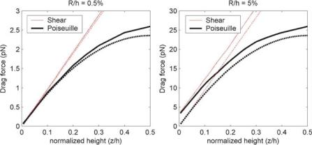
A B

FIGURE 8.4. Drag force using different approximations for a particle that is 0.5% (A) and 5% (B) of the chamber height. For the smaller particle (A), all approaches give the same result near the surface. For larger particles (B), the exact formulations (—) give better results than approximate approaches (- - -).

derived by numerical modeling. In that case one can compute the Stokes’ drag at each point by multiplying Eqn. (8.15) with the computed 3-D velocity field. To get a more exact result, especially for particles that are near walls, one can turn to solved examples in the fluid mechanics literature. Of special interest to trapping particles, the drag force on both a stationary and moving sphere near a wall in both plane Poiseuille [19] and shear flow [26] has been solved. The calculated drag forces have the same form as Eqn (8.15) but include a non-dimensional multiplying factor that accounts for the presence of the wall.

In Figure 8.4 I compare drag forces on 1 µm and 10 µm-diameter spheres using the different formulations. In both cases, the channel height is fixed at 100 µm. One sees two very different behaviors. When the sphere size is small compared to the channel height (R = 0.5% of h), all four formulations give similar results near the chamber wall (Figure 8.4A), with the anticipated divergence of the shear and Poiseuille drag profiles away from the wall. However, as the sphere becomes larger compared to the chamber height (Figure 8.4B), the different formulations diverge. Both the shear and parabolic profiles calculated using a single approach converge to identical values at the wall, but the two approaches yield distinctly different results. In this regime the drag force calculated using Eqn. (8.15) consistently underestimates the drag force, in this case by about 2 pN. This has a profound effect near the wall, where the actual drag force is 50% higher than that estimated by the simple approximation. Thus, for small particles (R h) away from walls (z R), the simple approximation is fine to within better than 10%, while in other cases one should use the exact formulations.

While spheres approximate most unattached mammalian cells as well as yeast and many bacteria, other cells (e.g., E. coli, erythrocytes) are aspherical. For these particles, drag forces have the same form as Eqn. (8.15) except that term 6π η R is replaced by different “friction” factors, nicely catalogued by Morgan and Green [60].

8.2.3.3. Electrothermal Forces The spatially non-uniform temperature distribution created by the power dissipated by the electric field can lead to flows induced by

electrothermal effects. These effects are covered in great detail by Morgan and Green [60]. Briefly, because the medium permittivity and conductivity are functions of temperature, temperature gradients directly lead to gradients in ε and σ . These gradients in turn generate free charge which can be acted upon by an electric field to move and drag fluid along with it, creating fluid flow. This fluid flow creates a drag force on an immersed body just as it does for conventional Stokes’ drag (Eqn. (8.15)). In general, derivations of the electrothermal force density, the resulting liquid flow, and the drag require numerical modeling because the details of the geometry profoundly impact the results. Castellanos et al. have derived solutions for one simple geometry, and have used it to great effect to derive some scaling laws [6].

8.3. DESIGN FOR USE WITH CELLS

Since dielectrophoretic cell manipulation exposes cells to strong electric fields, one needs to know how these electric fields might affect cell physiology. Ideally, one would like to determine the conditions under which the trapping will not affect the cells and use those conditions to constrain the design. Of course, cells are poorly understood complex systems and thus it is impossible to know for certain that one is not perturbing the cell. However, all biological manipulations—cell culture, microscopy, flow cytometer, etc.—alter cell physiology. What’s most important is to minimize known influences on cell behavior and then use proper controls to account for the unknown influences. In short, good experimental design.

The known influences of electric fields on cells can be split into the effects due to current flow, which causes heating, and direct interactions of the fields with the cell. We’ll consider each of these in turn.

8.3.1. Current-Induced Heating

Electric fields in a conductive medium will cause power dissipation in the form of Joule heating. The induced temperature changes can have many effects on cell physiology. As mentioned previously, microscale DEP is advantageous in that it minimizes temperature rises due to dissipated power. However, because cells can be very sensitive to temperature changes, it is not assured that any temperature rises will be inconsequential.

Temperature is a potent affecter of cell physiology [4, 11, 55, 75]. Very high temperatures (>4 ◦C above physiological) are known to lead to rapid mammalian cell death, and research has focused on determining how to use such knowledge to selectively kill cancer cells [81]. Less-extreme temperature excursions also have physiological effects, possibly due to the exponential temperature dependence of kinetic processes in the cell [93]. One well-studied response is the induction of the heat-shock proteins [4, 5]. These proteins are molecular chaperones, one of their roles being to prevent other proteins from denaturing when under environmental stresses.

While it is still unclear as to the minimum temperature excursion needed to induce responses in the cell, one must try to minimize any such excursions. A common rule of thumb for mammalian cells is to keep variations to <1 ◦C, which is the approximate daily variation in body temperature [93]. The best way we have found to do this is to numerically solve for the steady-state temperature rise in the system due to the local heat sources given by σ E2. Convection and radiation can usually be ignored, and thus the problem reduces to

solving for the conduction heat flow subject to the correct boundary conditions. Then, using the scaling of temperature rise with electric field and fluid conductivity (Eqn. (8.13)), one can perform a parametric design to limit temperature rises.

8.3.2. Direct Electric-Field Interactions

Electric fields can also directly affect the cells. The simple membrane-covered sphere model for mammalian cells can be used to determine where the fields exist in the cell as the frequency is varied. From this one can determine likely pathways by which the fields could impact physiology [31, 73]. Performing the analysis indicates that the imposed fields can exist across the cell membrane or the cytoplasm. A qualitative electrical model of the cell views the membrane as a parallel RC circuit connected in-between RC pairs for the cytoplasm and the media. At low frequencies (<MHz) the circuit looks like three resistors in series and because the membrane resistance is large the voltage is primarily dropped across it. This voltage is distinct from the endogenous transmembrane potential that exists in the cell. Rather, it represents the voltage derived from the externally applied field. The total potential difference across the cell membrane would be given by the sum of the imposed and endogenous potentials. At higher frequencies the impedance of the membrane capacitor decreases sufficiently that the voltage across the membrane starts to decrease. Finally, at very high frequencies (100’s MHz) the model looks like three capacitors in series and the membrane voltage saturates.

Quantitatively, the imposed transmembrane voltage can be derived as [73]

1.5|E|R

|Vt m | = (8.18) 1 + (ωτ )2

where ω is the radian frequency of the applied field and τ is the time constant given by

where ρcyt o and ρmed med are the cytoplasmic and medium resistivities ( -m). At low frequencies |Vm | is constant at 1.5|E|R but decreases above the characteristic frequency (1/τ ). This model does not take into account the high-frequency saturation of the voltage, when the equivalent circuit is a capacitive divider.

At the frequencies used in DEP—10’s kHz to 10’s MHz—the most probably route of interaction between the electric fields and the cell is at the membrane [79]. There are several reasons for this. First, electric fields already exist at the cell membrane, leading to transmembrane voltages in the 10’s of millivolts. Changes in these voltages could affect voltage-sensitive proteins, such as voltage-gated ion channels [7]. Second, the electric field across the membrane is greatly amplified over that in solution. From Eqn. (6.18) one gets that at low frequencies

1.5|E|R

|Vt m | = ≈ 1.5|E|R

1 + (ωτ )2

(8.20)

|Et m | ≈ |Vm |/t = (1.5R/t ) · |E|

174 JOEL VOLDMAN

and thus at the membrane the imposed field is multiplied by a factor of 1.5 R/t ( 1000), which can lead to quite large membrane fields (Et m ). This does not preclude effects due to cytoplasmic electric fields. However, these effects have not been as intensily studied, perhaps because 1) those fields will induce current flow and thus heating, which is not a direct interaction, 2) the fields are not localized to an area (e.g., the membrane) that is likely to have field-dependent proteins, and 3) unlike the membrane fields, the cytoplasmic fields are not amplified.

Several studies have investigated possible direct links between electric fields and cells. At low frequencies, much investigation has focused on 60-Hz electromagnetic fields and their possible effects, although the studies thus far are inconclusive [54]. DC fields have also been investigated, and have been shown to affect cell growth [44] as well as reorganization of membrane components [68]. At high frequencies, research has focused on the biological effects of microwave radiation, again inconclusively [65].

In the frequency ranges involved in DEP, there has been much less research. Tsong has provided evidence that some membrane-bound ATPases respond to fields in the kHz–MHz range, providing at least one avenue for interaction [79]. Electroporation and electrofusion are other obvious, although more violent, electric field-membrane coupling mechanisms [98].

Still other research has been concerned specifically with the effects of DEP on cells, and has investigated several different indicators of cell physiology to try to elucidate any effects. One of the first studies was by the Fuhr et al., who investigated viability, anchorage time, motility, cell growth rates, and lag times after subjecting L929 and 3T3 fibroblast cells in saline to short and long (up to 3 days) exposure to 30–60 kV/m fields at 10–40 MHz near planar quadrupoles [16]. They estimated that the transmembrane load was <20 mV. The fields had no discernable effect.

Another study investigated changes in cell growth rate, glucose uptake, lactate and monoclonal antibody production in CHO & HFN 7.1 cells on top of interdigitated electrodes excited at 10 MHz with 105 V/m in DMEM (for the HFN 7.1 cells) or serum-free medium (for the CHO cells) [12]. Under these conditions they observed no differences in the measured properties between the cells and control populations.

Glasser and Fuhr attempted to differentiate between heating and electric-field effects on L929 mouse fibroblast cells in RPMI to the fields from planar quadrupoles [24]. They imposed 40 kV/m fields of between 100 kHZ and 15 MHz for 3 days and observed monolayers of cells near the electrodes with a video microscopy setup, similar to their previous study [16]. They indirectly determined that fields of 40 kV/m caused an 2 ◦C temperature increase in the cells, but did not affect celldivision rates. They found that as they increased field frequency (from 500 kHZ to 15 MHz) the maximum tolerable field strength (before cell-division rates were altered) increased. This is consistent with a decrease in the transmembrane load with increasing frequency.

Wang et al. studied DS19 murine erythroleukemia cells exposed to fields ( 105 V/m) of 1 kHz–10 MHz in low-conductivity solutions for up to 40-min [90]. They found no effects due to fields above 10 kHz. They determined that hydrogen peroxide produced by reactions at the electrode interfaces for 1 kHz fields caused changes in cell growth lag phase, and that removal of the peroxide restored normal cell growth.

On the p-DEP side, Archer et al. subjected fibroblast-like BHK 21 C13 cells to p-DEP forces produced by planar electrodes arranged in a sawtooth configuration [1]. They used low-conductivity (10 mS/m) isoosmotic solutions and applied fields of 105 V/m at 5 MHz. They monitored cell morphology, cell doubling time, oxidative respiration (mitochondrial stress assay), alterations in expression of the immediate-early protein fos, and non-specific gene transcription directly after a 15 minute exposure and after a 30-min time delay. They observed 20–30% upregulation of fos expression and a upregulation of a few unknown genes (determined via mRNA analysis). Measured steady-state temperatures near the cells were <1 ◦C above normal, and their calculated transmembrane voltage under their conditions was <100 µV, which should be easily tolerable. The mechanism— thermal or electrical—of the increased gene expression was left unclear. It is possible that artifacts from p-DEP attraction of the cells to the electrodes led to observed changes. Either way, this study certainly demonstrates the possibility that DEP forces could affect cell physiology.

Finally, Gray et al. exposed bovine endothelial cells in sucrose media (with serum) to different voltages—and thus fields—for 30-min in order to trap them and allow them to adhere to their substrates. They measured viability and growth of the trapped cells and found that cell behavior was the same as controls for the small voltages but that large voltages caused significant cell death [27]. This study thus demonstrates the p-DEP operation in artificial media under the proper conditions does not grossly affect cell physiology.

In summary, studies specifically interested in the effects of kHz–MHz electroquasistatic fields on cells thus far demonstrate that choosing conditions under which the transmembrane loads and cell heating are small—e.g., >MHz frequencies, and fields in 10’s kV/m range—can obviate any gross effects. Subtler effects, such as upregulation of certain genetic pathways or activation of membrane-bound components could still occur, and thus DEP, as with any other assay technique, must be used with care.

8.4. TRAP GEOMETRIES

The electric field, which creates the DEP force, is in turn created by electrodes. In this section I will examine some of the electrode structures used in this field and their applicability to trapping cells and other microparticles. The reader is also encouraged to read the relevant chapters in Hughes’ [39] and Morgan and Green’s texts [60], which contain descriptions of some field geometries.

One can create traps using either p-DEP or n-DEP. Using n-DEP a zero-force point is created away from electrodes at a field minimum and the particle is trapped by pushing at it from all sides. In p-DEP the zero-force point is at a field maximum, typically at the electrode surface or at field constrictions. Both approaches have distinct advantages and disadvantages, as outlined in Table 8.2. For each application, the designer must balance these to select the best approach.

8.4.1. n-DEP Trap Geometries

Although an infinite variety of electrode geometries can be created, the majority of research has focused on those that are easily modeled or easily created.