

Biomolecular Sensing Processing and Analysis - Rashid Bashir and Steve Wereley
.pdf156 |
ABRAHAM P. LEE, JOHN COLLINS, AND ASUNCION V. LEMOFF |
particles migrate at different rates in the applied field, reaching different positions in the parabolic flow profile. Continuous separation of analytes performed by free-flow electrophoresis (FFE) where a mixture of charged particles is continuously injected into the carrier stream flowing between two electrode plates. When an electric field is applied, the particles are deflected from the direction of flow according to their electrophoretic mobility or pI.
In a microfluidic transverse isoelectric focusing device [13] two walls of the channels are formed by gold or palladium electrodes. The electrodes were in direct contact with the solution, so that the acid and base generated as a result of water electrolysis; OH− at the cathode, and H+ at the anode, can be exploited to form the pH gradient. The partial pressures of oxygen and hydrogen gases also produced by electrolysis could be kept below the threshold of bubble formation by keeping the voltages low, so no venting is required. Both acid-base indicators and protein conjugated with fluorescent dyes with experimentally determined pI values are used to monitor the formation of the pH gradients in the presence of pressure-driven flow. The micro IEF technique is utilized to separate and concentrate subcellular organelles (eg. Nuclei, peroxisomes, and mitochondria) from crude cell lysate [20].
7.5. SUMMARY
There are two types of integrated microfluidic devices for micro total analysis systems (µTAS): passive flow through devices and active programmable devices. The former (passive) devices are designed specifically for certain fixed biological and chemical assays where process steps are sequential in flow-through configurations. One example is described in [2] where mixing, reaction, separation, and self-calibration of immunoassays are performed on a microchip. The advantages of passive devices include reduced need for valves, simplified design, and likely higher manufacturing yield. On the other hand, passive devices are limited to fixed, predetermined assays, and are more difficult to design for multi-analyte detection. Active programmable microfluidic devices are more difficult to design and fabricate since they require integrated microvalves and micropumps. However,
MHD pump electrode pair
FIGURE 7.20. Illustration of complex fluidic routing on an integrated chip-scale platform using microchannel parallel electrodes enabling truly integrated, programmable “lab-on-a-chip”.
A MULTI-FUNCTIONAL MICRO TOTAL ANALYSIS SYSTEM (µTAS) PLATFORM |
157 |
active devices such as those implemented by the microchannel parallel electrodes platform are programmable, reconfigurable, and have the potential to become universal modules for biochemical processes.
Applications of MHD microfluidics are abundant. MHD-based microfluidic switching can route samples/reagents into different detection systems. Programmable combinatorial chemistry and biology assays can be implemented by a generic MHD microfluidic control platform. Local pumps can enable the integration of diffusion-based assays [30], flow cytometry, micro titration, or sample extractors. Ultimately the most powerful implementation of MHD-based microfluidics will be a general platform as shown in Fig. 7.20 for the design of new chemical and biological assays with few limits on complexity.
REFERENCES
[1]K. Asami, E. Gheorghiu, and T. Yonezawa. Real-time monitoring of yeast cell division by dielectric spectroscopy. Biophys. J., 76:3345–3348, 1999.
[2]S. Attiya, X.C. Qiu, G. Ocvirk, N. Chiem, W.E. Lee, and D.J. Harrison. Integrated microsystem for sample introduction, mixing, reaction, separation and self calibration. In D.J.H. a. A. v. d. Berg, (ed.) Micro Total Analysis Systems ’98, Kluwer Academic Publishers, Dordrecht,Banff, Canada, pp. 231–234, 1998.
[3]H.E. Ayliffe, A.B. Frazier, and R.D. Rabitt. Electrical impedance spectroscopy using microchannels with integrated metal electrodes. IEEE J. MEMS, 8:50–57, 1999.
[4]R.S. Baker and M.J. Tessier. Handbook of Electromagnetic Pump Technology. Elsevier, New York, 1987.
[5]H.H. Bau. A case for magneto-hydrodynamics (MHD). In J.A. Shaw and J. Main, (eds.), International Mechanical Engineering Congress and Exposition, American Society of Mechanical Engineers, New York City, 2001.
[6]H.H. Bau, J. Zhong, and M. Yi. A minute magneto hydro dynamic (MHD) mixer. Sens. Actu. B, Chem., 79:207, 2001.
[7]J. Collins and A.P. Lee. Microfluidic flow transducer based on the measurement of electrical admittance. Lab. Chip., 4:7–10, 2004.
[8]D.C. Duffy, J.C. McDonald, O.J.A. Schueller, and G.M. Whitesides. Rapid prototyping of microfluidic systems in poly(dimethylsiloxane), Anal. Chem., 70:4974–4984, 1998.
[9]J.C.T. Eijkel, C. Dalton, C.J. Hayden, J.A. Drysdale, Y.C. Kwok, and A. Manz. Development of a micro system for circular chromatography using wavelet transform detection. In J.M.R. et. al. Micro Total Analysis Systems 2001, Kluwer Academic Publishers, Monterey, CA, pp. 541–542, 2001.
[10]A.C. Fisher. Electrode Dynamics, Oxford University Press, Oxford, 1996.
[11]M.Y.J. Zhong and H.H. Bau. Magneto hydrodynamic (MHD) pump fabricated with ceramic tapes. Sens. Actu. A, Phys., 96:59–66, 2002.
[12]J. Jang and S.S. Lee. Theoretical and experimental study of MHD (magnetohydrodynamic) micropump. Sens. Actu. A, 80:84, 2000.
[13]K. Macounova, C.R. Cabrera, and P. Yager. Anal. Chem., Concentration and separation of proteins in microfluidic channels on the basis of transverse IEF 73:1627–1633, 2001.
[14]K.P.L.A. Christel, W. McMillan, and M.A. Northrup. Rapid, automated nucleic acid probe assays using silicon microstructures for nucleic acid concentration. J. Biomed. Eng., 121:22–27, 1999.
[15]A.V. Lemoff. Flow Driven Microfluidic Actuators for Micro Total Analysis Systems: Magnetohydrodynamic Micropump and Microfluidic Switch, Electrostatic DNA Extractor, Dielectrophoretic DNA Sorter, PhD Thesis, Dept. of Applied Science, UC Davis, 2000.
[16]A.V. Lemoff and A.P. Lee. An AC magnetohydrodynamic micropump. Sens. Actu. B, 63:178, 2000.
[17]A.V. Lemoff and A.P. Lee. Biomed. Microdev., 5(1); 55–60, 2003.
[18]V.G. Levich. Physicochemical Hydrodynamics, Prentice Hall, Englewood Cliffs, NJ, 1962.
[19]T.F. Lin and J.B. Gilbert. Analyses of magnetohydrodynamic propulsion with seawater for underwater vehicles, J. Propulsion, 7:1081–1083, 1991.
158 |
ABRAHAM P. LEE, JOHN COLLINS, AND ASUNCION V. LEMOFF |
[20]H. Lu, S. Gaudet, P.K. Sorger, M.A. Schmidt, and K.F. Jensen. Micro isoelectric free flow separation of subcellular materials. In M.A. Northrup, K.F. Jensen and D.J. Harrison, (eds.), 7th International Conference on Miniaturized Chemical and Biochemical Analysis Systems Squaw Valley, California, USA, pp. 915–918, 2003.
[21]S.K. Mohanty, S.K. Ravula, K. Engisch, and A.B. Frazier. Single cell analysis of bovine chromaffin cells using micro electrical impedance spectroscopy. In Y. Baba, A. Berg, S. Shoji, (eds.), 6th International Conference on Miniaturized Chemical and Biochemical Analysis Systems, Micro Total Analysis Systems, Nara, Japan, November 2002, Dordrecht, Kluwer Academic, 2002.
[22]W.J. Moore. Phys. Chem., Prentice-Hall, 1972.
[23]O.M. Phillips. The prospects for magnetohydrodynamic ship propulsion. J. Ship Res., 43:43–51, 1962.
[24]Y. Polevaya, I. Ermolina, M. Schlesinger, B.Z. Ginzburg, and Y. Feldman. Time domain dielectric spectroscopy study of human cells: II. Normal and malignant white blood cells. Biochim. Biophys. Acta, 15:257– 271, 1999.
[25]J.I. Ramos and N.S. Winowich. Magnetohydrodynamic channel flow study. Phys. Fluids, 29:992–997, 1986.
[26]R.B.M. Schasfoort, R. Luttge,¨ and A. van den Berg. Magneto-hydrodynamically (MHD) directed flow in microfluidic networks. In J.M. Ramsey. Micro Total Analysis Systems 2001. Kluwer Academic Publishers, Monterey, CA, pp. 577–578, 2001.
[27]L.L. Sohn, O.A. Saleh, G.R. Facer, A.J. Beavis, R.S. Allan, and D.A. Notterman. PNAS, 97:10687–10690, 2000.
[28]K.Y. Tam, J.P. Larsen, B.A. Coles, and R.G. Compton. J. Electroanal. Chem., 407:23–35, 1996.
[29]S. Way and C. Delvin. AIAA, 67:432, 1967.
[30]B.H. Weigl and P. Yager. Science, 15:346–347, 1999.
[31]F.M. White. Fluid Mech., McGraw-Hill, 1979.
[32]Y. Xia, E. Kim, and G.M. Whitesides. Chem. Mater., 8:1558–1567, 1996.
8
Dielectrophoretic Traps for
Cell Manipulation
Joel Voldman
Department of Electrical Engineering, Room 36-824, Massachusetts Institute of Technology Cambridge, MA 02139
8.1. INTRODUCTION
One of the goals of biology for the next fifty years is to understand how cells work. This fundamentally requires a diverse set of approaches for performing measurements on cells in order to extract information from them. Manipulating the physical location and organization of cells or other biologically important particles is an important part in this endeavor. Apart from the fact that cell function is tied to their three-dimensional organization, one would like ways to grab onto and position cells. This lets us build up controlled multicellular aggregates, investigate the mechanical properties of cells, the binding properties of their surface proteins, and additionally provides a way to move cells around. In short, it provides physical access to cells that our fingers cannot grasp.
Many techniques exist to physically manipulate cells, including optical tweezers [78], acoustic forces [94], surface modification [52], etc. Electrical forces, and in particular dielectrophoresis (DEP), are an increasingly common modality for enacting these manipulations. Although DEP has been used successfully for many years to separate different cell types (see reviews in [20, 38]), in this chapter I focus on the use of DEP as “electrical tweezers” for manipulating individual cells. In this implementation DEP forces are used to trap or spatially confine cells, and thus the chapter will focus on creating such traps using these forces. While it is quite easy to generate forces on cells with DEP, it is another thing altogether to obtain predetermined quantitative performance. The goal for this chapter is to help others develop an approach to designing these types of systems. The focus will be on trapping cells—which at times are generalized to “particles”—and specifically mammalian
160 |
JOEL VOLDMAN |
cells, since these are more fragile than yeast or bacteria and thus are in some ways more challenging to work with.
I will start with a short discussion on what trapping entails and then focus on the forces relevant in these systems. Then I will discuss the constraints when working with cells, such as temperature rise and electric field exposure. The last two sections will describe existing trapping structures as well as different approaches taken to measure the performance of those structures. The hope is that this overview will give an appreciation for the forces in these systems, what are the relevant design issues, what existing structures exist, and how one might go about validating a design. I will not discuss the myriad other uses of dielectrophoresis; these are adequately covered in other texts [39, 45, 60] and reviews.
8.2. TRAPPING PHYSICS
8.2.1. Fundamentals of Trap Design
The process of positioning and physically manipulating particles—cells in this case— is a trapping process. A trap uses a set of confining forces to hold a particle against a set of destabilizing forces. In this review, the predominant confining force will be dielectrophoresis, while the predominant destabilizing forces will be fluid drag and gravity. The fundamental requirement for any deterministic trap is that it creates a region where the net force on the particle is zero. Additionally, the particle must be at a stable zero, in that the particle must do work on the force field in order to move from that zero [3]. This is all codified in the requirement that Fnet = 0, Fnet · dr < 0 at the trapping point, where Fnet is the net force and dr is an increment in any direction.
The design goal is in general to create a particle trap that meets specific requirements. These requirements might take the form of a desired trap strength or maximum flowrate that trapped particles can withstand, perhaps to meet an overall system throughput specification. For instance, one may require a minimum flowrate to replenish the nutrients around trapped cells, and thus a minimum flowrate against which the cells must be trapped. When dealing with biological cells, temperature and electric-field constraints are necessary to prevent adverse effects on cells. Other constraints might be on minimum chamber height or width—to prevent particle clogging—or maximum chamber dimensions—to allow for proximate optical access. In short, predictive quantitative trap design. Under the desired operating conditions, the trap must create a stable zero, and the design thus reduces to ensuring that stable zeros exist under the operating conditions, and additionally determining under what conditions those stable zeros disappear (i.e., the trap releases the particle).
Occasionally, it is possible to analytically determine the conditions for stable trapping. When the electric fields are analytically tractable and there is enough symmetry in the problem to make it one-dimensional, this can be the best approach. For example, one can derive an analytical expression balancing gravity against an exponentially decaying electric field, as is done for field-flow fractionation [37]. In general, however, the fields and forces are too complicated spatially for this approach to work. In these cases, one can numerically calculate the fields and forces everywhere in space and find the net force (Fnet) at each point, then find the zeros.
DIELECTROPHORETIC TRAPS FOR CELL MANIPULATION |
161 |
A slightly simpler approach exists when the relevant forces are conservative. In this case one can define scalar potential energy functions U whose gradient gives each force (i.e., F = −U ). The process of determining whether a trap is successfully confining the particle then reduces to determining whether any spatial minima exist within the trap. This approach is nice because energy is a scalar function and thus easy to manipulate by hand and on the computer.
In general, a potential energy approach will have limited applicability because dissipation is usually present. In this case, the energy in the system depends on the specifics of the particle motion—one cannot find a U that will uniquely define F. In systems with liquid flow, for example, an energy-based design strategy cannot be used because viscous fluid flow is dissipative. In this case, one must use the vector force-fields and find stable zeroes.
In our lab, most modeling incorporates a range of approaches spanning analytical, numerical, and finite-element modeling. In general, we find it most expedient to perform finite-element modeling only when absolutely necessary, and spend most of the design combining those results with analytical results in a mixed-numerical framework run on a program such as Matlab c (Mathworks, Natick, MA). Luckily, one can run one or two finite-element simulations and then use simple scaling laws to scale the resulting data appropriately. For instance, the linearity of Laplace’s equation means that after solving for the electric fields at one voltage, the results can be linearly scaled to other voltages. Thus, FEA only has to be repeated when the geometry scales, if at all.
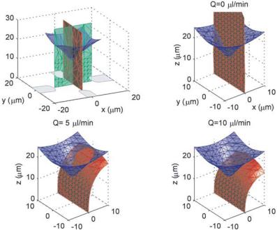
To find the trapping point (and whether it exists), we use MATLAB to compute the three isosurfaces where each component of the net force (Fx , Fy , Fz ) is zero. This process is shown in Figure 8.1 for a planar quadrupole electrode structure. Each isosurface—the three-dimensional analog of a contour line—shows where in space a single component of the force is zero. The intersection of all three isosurfaces thus represents points where all three force components, and thus the net force, is zero. In the example shown in Figure 8.1,B– D, increasing the flowrate changes the intersection point of the isosurfaces, until at some threshold flowrate (Figure 8.1D), the three isosurfaces cease to intersect, and the particle is no longer held; the strength of the trap has been exceeded [83]. In this fashion we can determine the operating characteristics (e.g., what voltage is needed to hold a particular cell against a particular flow) and then whether those characteristics meet the system requirements (exposure of cells to electric fields, for instance).
A few caveats must be stated regarding this modeling approach. First, the problem as formulated is one of determining under what conditions an already trapped particle will remain trapped; I have said nothing about how to get particles in traps. Luckily this is not a tremendous extension. Particle inertia is usually insignificant in microfluidic systems, meaning that particles will follow the streamlines of the force field. Thus, with numerical representations of the net force, one can determine, given a starting point, where that particle will end up. Matlab in fact has several commands to do this (e.g., streamline). By placing test particles in different initial spots, it is possible to determine the region from within which particles will be drawn to the trap.
Another implicit assumption is that only one particle will be in any trap, and thus that particle-particle interactions do not have to be dealt with. In actuality, designing a trap that will only hold one particle is quite challenging. To properly model this, one must account for the force perturbations created when the first particle is trapped; the second particle sees a force field modified by the first particle. While multiple-particle modeling is still largely
162 JOEL VOLDMAN
A B
C D
FIGURE 8.1. Surfaces of zero force describe a trap. (A) Shown are the locations of planar quadrupole electrodes along with the three isosurfaces where one component of the force on a particle is zero. The net force on the particle is zero where the three surfaces intersect. (B–D) As flow increases from left to right, the intersection point moves. The third isosurface is not shown, though it is a vertical sheet perpendicular to the Fx = 0 isosurface.
(D) At some critical flow rate, the three isosurfaces no longer intersect and the particle is no longer trapped.
unresolved, the single-particle approach presented here is quite useful because one can, by manipulating experimental conditions, create conditions favorable for single-particle trapping, where the current analysis holds.
Finally, we have constrained ourselves to deterministic particle trapping. While appropriate for biological cells, this assumption starts to break down as the particle size decreases past 1µm because Brownian motion makes trapping a probabilistic event. Luckily, as nanoparticle manipulation has become more prevalent, theory and modeling approaches have been determined. The interested reader is referred to the monographs by Morgan and Green [60] and Hughes [39].
8.2.2. Dielectrophoresis
The confining force that creates the traps is dielectrophoresis. Dielectrophoresis (DEP) refers to the action of a body in a non-uniform electric field when the body and the surrounding medium have different polarizabilities. DEP is easiest illustrated with reference to Figure 8.2. On the left side of Figure 8.2, a charged body and a neutral body (with different permittivity than the medium) are placed in a uniform electric field. The charged body feels a force, but the neutral body, while experiencing an induced dipole, does not feel a net
DIELECTROPHORETIC TRAPS FOR CELL MANIPULATION |
163 |
|
Uniform Field |
|
Non-uniform Field |
|
|
|||||||||
A Charged |
|
-V |
|
|
F |
B |
|
|
|
|
Cell |
|||
body |
- |
|
|
|
|
|
+ |
|
|
|
-V |
|
|
|
|
|
++++ |
|
F |
|
|
Induced |
|||||||
|
- |
- |
+ ++ |
+ |
No |
|
|
+ |
||||||
|
|
|
|
|
|
|
+ |
|
Net |
|
||||
Net - |
- - |
|
|
|
|
|
Net |
++ |
|
- |
dipole |
|||
|
|
- |
|
- |
+++ |
|
Force |
|||||||
Force |
|
|
|
- |
|
Force |
+ + |
|
|
|||||
|
- |
|
- |
|
-- |
|
|
- |
|
|
|
|||
|
|
Neutral |
--- |
|
|
|
|
|
|
|||||
|
|
|
|
|
|
|
|
|
|
|
- |
|
|
Electric |
|
|
|
|
body |
|
|
F |
|
--- |
|
|
|||
|
|
F- |
|
|
|
--- |
|
F- |
|
field |
||||
|
|
|
|
|
|
- |
|
|
|
|
||||
|
|
|
|
+V |
|
|
|
|
|
|
|
+V |
|
Electrodes |
|
|
|
|
|
|
|
|
|
|
|
|
|
||
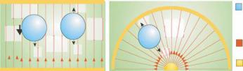
FIGURE 8.2. Dielectrophoresis. The left panel (A) shows the behavior of particles in uniform electric fields, while the right panel shows the net force experienced in a non-uniform electric field (B).
force. This is because each half of the induced dipole feels opposite and equal forces, which cancel. On the right side of Figure 8.2, this same body is placed in a non-uniform electric field. Now the two halves of the induced dipole experience a different force magnitude and thus a net force is produced. This is the dielectrophoretic force.
The force in Figure 8.2, where an induced dipole is acted on by a non-uniform electric field, is given by [45]
Fdep = 2π εm R3Re[C M(ω)] · |E(r)|2 |
(8.1) |
where εm is the permittivity of the medium surrounding the particle, R is the radius of the particle, ω is the radian frequency of the applied field, r refers to the vector spatial coordinate, and E is the applied vector electric field. The Clausius-Mossotti factor (CM)—CM factor— gives the frequency (ω) dependence of the force, and its sign determines whether the particle experiences positive or negative DEP. Importantly, the above relation is limited to instances where the field is spatially invariant, in contrast to traveling-wave DEP or electrorotation (see [39, 45]).
Depending on the relative polarizabilities of the particle and the medium, the body will feel a force that propels it toward field maxima (termed positive DEP or p-DEP) or field minima (negative DEP or n-DEP). In addition, the direction of the force is independent of the polarity of the applied voltage; switching the polarity of the voltage does not change the direction of the force—it is still toward the field maximum in Figure 8.2. Thus DEP works equally well with both DC and AC fields.
DEP should be contrasted with electrophoresis, where one manipulates charged particles with electric fields [30], as there are several important differences. First, DEP does not require the particle to be charged in order to manipulate it; the particle must only differ electrically from the medium that it is in. Second, DEP works with AC fields, whereas no net electrophoretic movement occurs in such a field. Thus, with DEP one can use AC excitation to avoid problems such as electrode polarization effects [74] and electrolysis at electrodes. Even more importantly, the use of AC fields reduces membrane charging of biological cells, as explained below. Third, electrophoretic systems cannot create stable non-contact traps, as opposed to DEP—one needs electromagnetic fields to trap charges (electrophoresis can, though, be used to trap charges at electrodes [63]). Finally, DEP forces increase with the square of the electric field (described below), whereas electrophoretic forces increase linearly with the electric field.

164 |
JOEL VOLDMAN |
This is not to say that electrophoresis is without applicability. It is excellent for transporting charged particles across large distances, which is difficult with DEP (though travelingwave versions exist [17]). Second, many molecules are charged and are thus movable with this technique. Third, when coupled with electroosmosis, electrophoresis makes a powerful separation system, and has been used to great effect [30].
8.2.2.1. The Clausius-Mossotti Factor The properties of the particle and medium within which it resides are captured in the form of the Clausius-Mossotti factor (CM)—CM factor. The Clausius-Mossotti factor arises naturally during the course of solving Laplace’s equation and matching the boundary conditions for the electric field at the surface of the particle (for example, see [45]). For a homogeneous spherical particle, the CM factor is given by
ε p − εm |
(8.2) |
C M = ε p + 2εm |
where εm and ε p are the complex permittivities of the medium and the particle, respectively,
and are each given by ε = ε + σ/( j ω), where ε is the permittivity of the medium or particle,
√
σ is the conductivity of the medium or particle, and j is −1.
Many properties lie within this simple relation. First, one sees that competition between the medium (εm ) and particle (ε p ) polarizabilities will determine the sign of CM factor, which will in turn determine the sign—and thus direction—of the DEP force. For instance, for purely dielectric particles in a non-conducting liquid (σp = σm = 0), the CM factor is purely real and will be positive if the particle has a higher permittivity than the medium, and negative otherwise.
Second, the real part of the CM factor can only vary between +1 (ε p εm , e.g., the particle is much more polarizable than the medium) and −0.5 (ε p εm , e.g., the particle is much less polarizable than the medium). Thus n-DEP can only be half as strong as p-DEP. Third, by taking the appropriate limits, one finds that at low frequency the CM
factor (Eqn. (8.2)) reduces to |
|
|
|
|
|
C M |
= |
|
σp − σm |
(8.3) |
|
σp + 2σm |
|||||
ω→0 |
|
||||
while at high frequency it is |
|
|
|
|
|
C M |
= |
|
εp − εm |
(8.4) |
|
|
εp + 2εm |
||||
ω→∞ |
|
|
|||
Thus, similar to many electroquasistatic systems, the CM factor will be dominated by relative permittivities at high frequency and conductivities at low frequencies; the induced dipole varies between a free charge dipole and a polarization dipole. The relaxation time separating the two regimes is
τ |
M W = |
εp + 2εm |
(8.5) |
|
σp + 2σm |
||||
|
|
DIELECTROPHORETIC TRAPS FOR CELL MANIPULATION |
165 |
1
|
0.5 |
|
|
|
(B) |
|
|
|
|
|
|
|
|
|
|
|
|
CM factor |
0 |
|
|
|
|
|
|
|
|
|
|
|
(C) |
|
|
|
|
|
−0.5 |
|
|
(A) |
|
|
|
|
|
|
|
|
|
|
|
||
|
|
|
|
|
|
|
|
|
|
103 |
104 |
105 |
106 |
107 |
108 |
||
frequency (Hz)
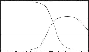
FIGURE 8.3. CM factor for three situations. (A) A non-conducting uniform sphere with ε p = 2.4 in nonconducting water (εm = 80). The water is much more polarizable than the sphere, and thus the CM factor is−0.5. (B) The same sphere, but with a conductivity σ p = 0.01 S/m in non-conducting water. Now there is one dispersion—at low frequencies the bead is much more conducting than the water & hence there is p-DEP, while at high frequencies the situation is as in (A). (C) A spherical shell (approximating a mammalian cell), with (εcyt o = 75, cm = 1 µF/cm2, σcyt o = 0.5 S/m, gm = 5 mS/cm2) in a 0.1 S/m salt solution, calculated using results from [45]. Now there are two interfaces and thus two dispersions. Depending on the frequency, the shell can experience n-DEP or p-DEP.
and is denoted τM W to indicate that the physical origin is Maxwell-Wagner interfacial polarization [73].
This Maxwell-Wagner interfacial polarization causes the frequency variations in the CM factor. It is due to the competition between the charging processes in the particle and medium, resulting in charge buildup at the particle/medium interface. If the particle and medium are both non-conducting, then there is no charge buildup and the CM factor will be constant with no frequency dependence (Figure 8.3A). Adding conductivity to the system results in a frequency dispersion in the CM factor due to the differing rates of interfacial polarization at the sphere surface (Figure 8.3B).
While the uniform sphere model is a good approximation for plastic microspheres, it is possible to extend this expression to deal with more complicated particles such as biological cells, including non-spherical ones.
Multi-Shelled Particulate Models Because we are interested in creating traps that use DEP to manipulate cells, we need to understand the forces on cells in these systems. Luckily, the differences between a uniform sphere and a spherical cell can be completely encompassed in the CM factor; the task is to create an electrical model of the cell and then solve Laplace’s equation to derive its CM factor (a good review of electrical properties of cells is found in Markx and Davey [57]). The process is straightforward, though tedious, and has been covered in detail elsewhere [39, 43, 45]. Essentially, one starts by adding a thin shell to the uniform sphere and matches boundary conditions at now two interfaces,