Biomolecular Sensing Processing and Analysis - Rashid Bashir and Steve Wereley

350um

FIGURE 13.1. (a) Schematic view of experimental apparatus and (b) photo of apparatus.

Instruments Inc.). The flow rate could be adjusted and precautions were taken to avoid air bubbles. An HP 33120A arbitrary waveform generator was used as the AC signal source to produce sinusoidal signal with frequency specified at 1MHz.

13.1.2. Dielectrophoresis Background

Dielectrophoretic forces arise from a difference in induced dipole moments between a particle and a surrounding fluid medium caused by an alternating electric field. Differences in permittivity between two materials result in a net force which depends on the gradient of the electric field [11]. This force can be used to manipulate particles suspended in a fluid [5, 7, 11]. The DEP force can either attract or repel particles from regions of large field gradient. A particle with permittivity smaller than that of the suspension medium will be repelled from entering regions of increasing field density, as is the case for the device observed in this study. The equation for the time-averaged DEP force [5] is as follows:

This force depends on the volume of a particle, the relative permittivities of a particle and surrounding medium, and the absolute gradient of average electric field squared. The

Clausius-Mossotti factor fcm contains the permittivities and frequency dependence of the DEP force. The factor is defined by

where ε denotes a complex permittivity based on the conductivity and frequency of excitation. The subscripts m and p denote properties related to a medium and particle respectively. The complex permittivity of the medium is given as

where σ and ω represent conductivity and angular frequency, respectively. The form of Eq. 13.3 is analogous for the complex permittivity of a particle. The conductivity of the particles used in this study, polystyrene microspheres, is approximately zero, thus ε p is equal to ε p which is found to be equal to 2.6.

Since the dielectrophoretic force scales with the cube of particle size, it is effective for manipulating particles of order one micron or larger. DEP has been used to separate blood cells and to capture DNA molecules [9, 12]. DEP has limited effectiveness for manipulating proteins that are of order 10–100 nm [3]. However, for these small particles, DEP force may be both augmented and dominated by the particle’s electrical double layer, particularly for low conductivity solutions [4]. DEP has been used to manipulate macromolecules and cells in microchannels. For example, Miles et al. [9] used DEP to capture DNA molecules in microchannel flow. Gascoyne & Vykoukal [4] presents a review of DEP with emphasis on manipulation of bioparticles.

13.1.3. Micro Particle Image Velocimetry

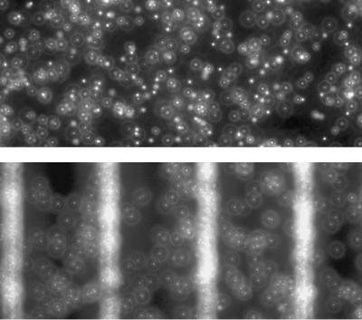
Images of the particles were acquired using a standard µPIV system. In these experiments a mercury lamp is used to illuminate the 0.7 µm polystyrene latex (PSL) microspheres (Duke Scientific) that are suspended in de-ionized water in concentrations of about 0.1%by volume. The particles are coated with a red fluorescing dye ( λabs = 542 nm, λemit = 612 nm). The images were acquired using a Photometrics CoolSNAP HQ interline transfer monochrome camera (Roper Scientific). This camera is capable of 65%quantum efficiency around the 610 nm wavelength. The largest available image size that can be accommodated by the CCD array is 1392 by 1040 pixels, but the camera has the capability of pixel binning, which can drastically increase the acquisition frame rate by reducing the number of pixels that need to be digitized. A three-by-three pixel binning scheme was used in this experiment, producing images measuring 464 by 346 pixels, which were captured at a speed of 20 frames per second. The average focused particle diameter in the images was approximately 3 pixels. Sample images are shown in Figure 13.2.

Shallow Channel Considerations When performing µPIV measurements on shallow microchannels, the depth of focus of the microscope can be comparable in size to the depth of the flow. A PIV cross-correlation peak, the location of which is the basis for conventional PIV velocity measurements, is a combination of the velocity distribution in the interrogation region and some function of average particle shape. PIV velocity measurements containing velocity gradients can substantially deviate from the ideal case of depthwise uniform flow.

FIGURE 13.2. A photo of PSL particles with 0.0 volts (top) and 4.0 (bottom).

Gradients within the light sheet plane have been addressed by image correction techniques [13], but gradients in the depthwise direction remain problematic. They can cause inaccurate velocity measurements due to the presence of multiple velocities within an interrogation region that are independent of mesh refinement. One problem with depthwise velocity gradients is cross-correlation peak deformation which reduces the signal to noise ratio of a PIV measurement [2]. Cross-correlation peak deformation can also reduce the effectiveness of subpixel peak fitting schemes which are based on a particular cross-correlation shape, such as a common five point Gaussian fit. There are both hardware and software approaches toward resolving these problems. In situations where a large in plane region must be imaged in a relatively thin device, the physics of the imaging system dictate that the entire depth of the channel will be focused. Hence a software approach must be used. Two different approaches are explored: deconvolving the cross correlation with the autocorrelation and image processing to replace the original particle images with unit impulse particle images.

13.2. MODELING/THEORY

13.2.1. Deconvolution Method

Simulated PIV experiments show a qualitative similarity between the cross-correlation function from a test flow containing velocity gradients in the depthwise direction and the

corresponding velocity histogram for that depthwise gradient, suggesting that the deconvolution procedure may work. The major hypothesis of the deconvolution method is that the PIV cross-correlation function can be approximated by the convolution of a particle image autocorrelation with the velocity distribution in the interrogation region. This hypothesis is based on observations of cross-correlations from experimental situations. For the case of a uniform flow, the velocity distribution is an impulse, and the resulting cross-correlation can be approximated by a position-shifted autocorrelation. This suggests that the crosscorrelation can be approximated by a convolution of the impulse velocity distribution and an image autocorrelation.

Olsen and Adrian [10] approximated the cross-correlation as a convolution of mean particle intensity, a fluctuating noise component, and a displacement component. Deconvolution of a cross-correlation with an autocorrelation is used by Cummings (1999) to increase the signal-to-noise ratio for a locally uniform flow. The new idea is to extract velocity distributions by deconvolving a PIV cross-correlation function with its autocorrelation. The result is a two-dimensional approximation of the underlying velocity distribution. One drawback to deconvolution procedures is sensitivity to noise resulting from a division operation in frequency space. Thus, it is important to have high information density in both the crosscorrelation and autocorrelation. The information density can be increased by correlation averaging both the cross-correlation and autocorrelation [8].

13.2.2. Synthetic Image Method

Since deconvolution is inherently sensitive to noise, it would be beneficial to eliminate the deconvolution step from the velocity profile extraction process. This could be done if the autocorrelation were an impulse or delta function. Since the deconvolution of a function with an impulse is the original function, this would render the deconvolution operation trivial and unnecessary.

The autocorrelation is related to the particle intensity distributions from a set of PIV recordings, i.e. the shape of particles in an image pair. So, the most practical way to affect the autocorrelation is to alter the imaged shape of these particles. If the particle intensity distributions in a set of PIV recordings are reduced to single pixel impulses, the autocorrelation appears as a single pixel impulse. This desirable autocorrelation trivializes the deconvolution method such that the cross-correlation alone is equal to the deconvolution of the cross-correlation and the autocorrelation. This is the basis for the synthetic image method.

Experimentally PIV recordings containing uniformly illuminated single pixel particle images can be approximately obtained by illuminating very small seed particles with a high intensity laser sheet, such that most particles are imaged by a single pixel by a digital camera. However, this approach can only be an approximation because even very small particles located near the edge of a pixel would be imaged over two neighboring pixels. Furthermore, in µPIV the particles are already very small, so making them any smaller could render them invisible to the camera; imaged particle intensity decreases proportionally as the cube of particle radius. Also, the image of a very small particle is dominated by diffraction optics, thus reducing the physical particle size will have very little impact on the imaged particle size due to a finite diffraction limited spot size. The typical point response function

associated with microscope objectives used in µPIV is 5 pixels, so the desired particle intensity distribution cannot easily be obtained in raw experimental images.

13.2.3. Comparison of Techniques

Three cases were examined to compare and validate the two methods of velocity distribution extraction from cross-correlation PIV. The cases involve three different velocity profiles that are frequently encountered in µPIV. The first is a uniform flow (depth of field small compared to flow gradients), the second is a linear shear (near wall region of a channel flow), and the third is a parabolic channel flow (depth averaged pressure-driven flow in a shallow micro device).

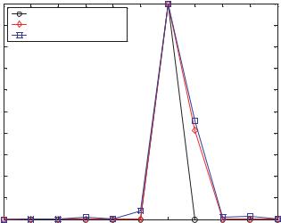
Uniform Flow The velocity profile of uniform flow is an ideal situation for making accurate PIV measurements. This case also has the simplest velocity histogram, a delta function at the uniform velocity value. The uniform one dimensional velocity profile simulated in this case study is given by Vx = 6.294. Both the deconvolution and the synthetic image methods generate the expected histograms and are shown in Figure 13.3. Since the histograms are calculated only at integer pixel values, they both show a peak at 6 pixels and a lower, but non-zero value at 7 pixels. By taking the average of the histogram values at 6 and 7 pixels, the true value of the uniform displacement can be found. For example in the case of the synthetic image method, Vx ,mean = (6 × 1 + 7 × 0.46)/1.46 = 6.32, which is very near the input value of 6.294.

Linear Shear Another common flow profile is a linear shear. In microfluidics, this type of flow can be seen in the near wall region of a parabolic flow profile. Since the

displacement probability density function for a linear shear has the simple shape of a top hat, this type of flow presents a good case to further benchmark the methods of deconvolution and synthetic images. This simulation case study used the velocity profile given by Vx = 6.294 × Z + 1.248 where Z is the position along the axis of the imaging system and can assume values between 0 and 1. Consequently we expect a top hat with the left edge at 1.248 and the right edge at 7.552. The results are plotted in Figure 13.4. The synthetic image method is a slightly better predictor of the velocity histogram than the deconvolution method by virtue of the steeper gradients at the edges of the distribution. This behavior is expected because images analyzed by deconvolution contain particle diameter and particle intensity variations, as well as slight readout noise.

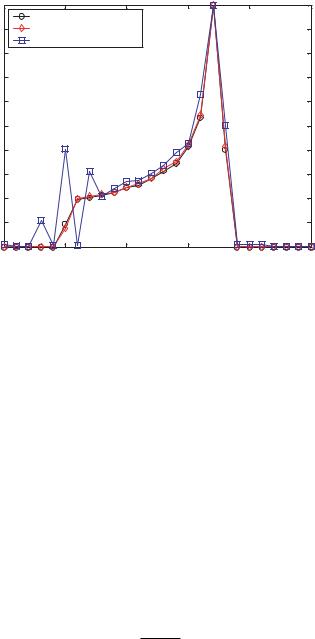
Parabolic or Poiseuille Flow The final common velocity profile to be considered is parabolic or Poiseuille flow. This type of flow is found in pressure-driven microchannel devices. Furthermore, it is the profile expected from the LOC experimental device being considered here with zero voltage applied to the DEP electrodes. This simulation used the velocity profile is given by Vx = 50.352 × (Z − Z 2), with Z varying between 0 and 1. Hence, we expect a velocity distribution varying between a minimum of 0 pixels at Z = 0 and Z = 1 and a maximum of 12.558 at Z = 1/2. The results are plotted in Figure 13.5. These results clearly show the increased accuracy of the synthetic image method over the deconvolution method. The synthetic image data very closely agrees with the velocity histogram. The deconvolution method suffers spurious oscillations but still gives a reasonable approximation of the velocity histogram. These spurious oscillations were initially attributed to a lack of statistical convergence, so additional image sets were added, eventually totaling ten thousand sets. The same spurious oscillations were found, so they must be inherent to this particular case. It is not typical for such oscillations to occur, but as demonstrated, the deconvolution method has definite limitations.

13.3. EXPERIMENTAL RESULTS

The experiments presented here are designed to quantify the dielectrophoretic performance of the device. The experiments used six sets of 800 images each to analyze the effect of dielectrophoresis on particle motion in the test device. These images are high quality with low readout noise, as can be seen in the example fluorescent image of Figure 13.6. The top image demonstrates the many different particle intensity distributions which are typically present in a µPIV image in which the particles are distributed randomly within the focal plane. The bottom figure shows how, as the result of the DEP force, the particles migrate to the top of the channel and all have nearly identical images. The top image also shows that when a significant DEP force exists, the particles are trapped at the electrode locations by the increase in DEP force there. In general, the observed particle image shape is the convolution of the geometric particle image with the point response function of the imaging system. The point response function of a microscope is an Airy function when the point being imaged is located at the focal plane. When the point is displaced from the focal plane, the Airy function becomes a Lommel function [1]. For a standard microscope the diffraction limited spot size is given by

A numerical aperture (or NA) of 1.00 and an incident light wavelength λ of 540nm results in a diffraction limited spot size of 0.66µm, while the particles used are 0.69µm. Consequently the particle intensity distributions as recorded by the camera are partly due to the geometric image of the particle and partly due to diffraction effects. Hence, the distance of any particle from the focal plane can be determined by the size and shape of the diffraction rings.

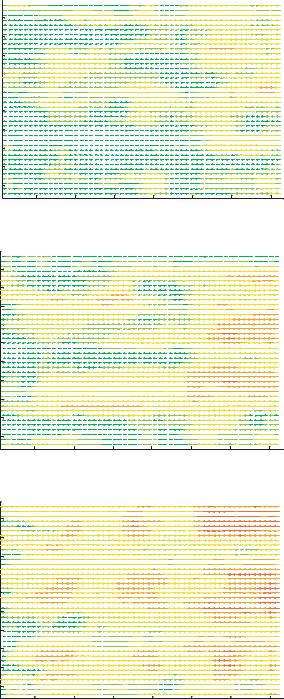
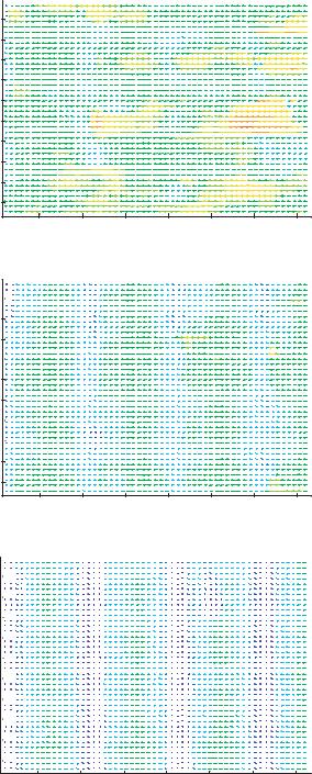
FIGURE 13.6. PIV vector plots for electrode voltages of a) 0.5 volts, b) 1.0 volts, c) 2.0 volts, d) 2.5 volts, e) 3.5 volts and f) 4.0 volts.

Conventional µPIV analysis Two different PIV analyses were performed. Initially a conventional µPIV analysis was performed to obtain an estimate of the average particle velocity field. Because the goal of the conventional µPIV analysis is not to extract velocity distribution, only the median velocity is reported. Figure 13.6 shows vector plots for the experimental cases ranging from 0.5 volts to 4.0 volts. A uniform color scale was applied among all the figures representing velocity magnitude, so that velocity changes between cases can be more easily interpreted. An interrogation region of 32 by 32 pixels and a grid spacing of 8 by 8 pixels were used. While this grid spacing over samples the data, it provides a good means of interpolating between statistically independent measurements. The advanced interrogation options included central difference interrogation (CDI), continuous window shifting (CWS), ensemble correlation averaging, and a multiple iteration scheme set to two passes. In all cases, the electrode voltage frequency was set to 580 kHz. This was determined by sweeping between frequencies of 100 kHz to 10MHz and qualitatively determining the most effective trapping frequency.

Velocity measurement statistics are reported in Table 13.1. The statistics show a maximum velocity of 27.5 microns/sec; this results in a Reynolds number of 3.3 10−4. The statistics also show that the average transverse velocity is negligible in comparison to axial velocities. A particle velocity increase can be observed as electrode voltage is increased from 0.5 volts to 2.0 volts. A velocity decrease is observed as electrode voltage is further increased from 2.0 volts to 4.0 volts. In the 2.5 volt case, low velocity regions between electrodes are first noticeable. In the 3.5 volt and 4.0 volt cases, large numbers of trapped particles result in near zero velocities.

The PIV results are summarized in Figure 13.7 which is a plot of the average axial velocities for the six electrode voltage cases. The three lowest voltages share a trend of decreasing particle velocity in the downstream direction. This phenomenon is evident in the curve fit parameters for linear slope given in Table 13.2. One explanation for this behavior may be that with each electrode a particle encounters, it lags the fluid velocity a little more. The cumulative effect results in a gradual slowing of the particle.

TABLE 13.1. PIV measurement statistics, all measurements are in (microns/second).