Biomolecular Sensing Processing and Analysis - Rashid Bashir and Steve Wereley

[28]W. Zhu, S.J. Singer, Z. Zheng, and A.T. Conlisk. Electroosmotic Flow of a Model Electrolyte. Phys. Rev., E 71(4):41501, 2005.

[29]A.J. Corkhill and L. Rosenhead. Distribution of Charge and Potential in an Electrolyte Bounded by Two Infinite Parallel Plates. Proc. Royal Soc., 172 (950):410, 1939.

[30]S. Levine and A. Suddaby. Simplified Forms for Free Energy of the Double Layers of Two Plates in a Symmetrical Electrolyte. Proc. Phys. Soc., A 64(3):287, 1951.

[31]H.J.C. Berendsen, J.P.M. Postma, W.F. von Gunsteren, and J. Hermans. Interaction Models for Water in Relation to Protein Hydration. In B. Pullman (ed.), Intermolecular Forces. Reidel, Dordrecht, Holland, p. 331, 1981.

[32]H.J.C. Berendsen, J.R. Grigera, and T.P. Straatsma. The Missing Term in Effective Pair Potentials. J. Phys. Chem., 91(24):6269, 1987.

[33]L. Onsager and N.N.T. Samaras. The Surface Tension of Debye-Huckel¨ Electrolytes. J. Chem. Phys., 2(8):1934.

[34]K.P. Travis and K.E. Gubbins. Poiseuille Flow of Lennard-Jones Fluids in Narrow Slit Pores. J. Chem. Phys., 112(4):1984, 2000.

16

Nano-Particle Image Velocimetry: A Near-Wall Velocimetry Technique with Submicron Spatial Resolution [1]

Minami Yoda [2]

16.1. INTRODUCTION

Over the last decade, characterizing and understanding fluid flow and transport at spatial scales of 100 µm or less has become a major area of research in fluid mechanics because of the rapid development of microscale devices based upon microelectromechanical systems (MEMS) fabrication techniques. Examples of such microfluidic devices include Labs-on-a-Chip for biochemical separation and analysis, inkjet printer heads, various types of microelectronic cooling devices, microscale fuel cells, microthrusters, and genomic and proteomic “chips”capable of sequencing and identifying various proteins including RNA and DNA. More recently, nanotechnology and the promise of engineering new devices at the molecular scale has sparked interest in understanding flow at spatial scales below 1µm. Optimizing and controlling the flow of liquids and gases in microand nanoscale devices requires both well-validated models of transport down to the molecular scale and diagnostic techniques with spatial resolution well below 1µm.

A major “bottleneck”in developing such flow models is our limited fundamental understanding of microscale flows and limitations in our ability to measure flow parameters such as velocity, pressure, concentration and temperature at these spatial scales. At the microscale, surface (vs. bulk) effects become significant; the new physical phenomena that may therefore be significant in microand nanoscale flows include apparent slip [3] (i.e., nonzero flow velocity at the wall due possibly to a “soft”dissociated fluid or gas layer [4, 5]); the effects of surface properties such as chemistry (e.g. hydrophobic vs. hydrophilic [6, 7]), molecular-scale roughness [8], and charge; and discrepancies in fluid properties (e.g.

viscosity) between the interfacial and bulk flow regions. Diagnostic techniques capable of interrogating the near-wall region to measure flow parameters within the first 100 nm of the wall are therefore important in understanding how surface effects impact microand nanoscale transport, and validating our current models of transport at these spatial scales.

This chapter first briefly reviews current experimental techniques in microfluidics, with an emphasis on velocimetry techniques and their spatial resolution and near-wall capabilities. The chapter then describes a new technique, nano-particle image velocimetry (nPIV), based upon evanescent-wave illumination generated by the total internal reflection of light at a refractive index interface. The applications of nPIV are illustrated by velocity and mobility results obtained in steady, fully-developed two-dimensional electroosmotic flow (EOF) of liquids.

16.2. DIAGNOSTIC TECHNIQUES IN MICROFLUIDICS

The majority of diagnostic techniques in fluid mechanics were originally developed for turbulent flows, where flow parameters such as velocity and pressure have strong stochastic fluctuations. “Classical”flow measurement diagnostic techniques such as hot-wire anemometry and laser-Doppler velocimetry (LDV) therefore emphasized measurements at a single spatial location with high temporal resolution or sampling rate. Over the last twenty years, advances in lasers and imaging technology have led to the development of a variety of nonintrusive optical diagnostic techniques for obtaining spatially and temporally resolved measurements of velocity and such as particle-image velocimetry (PIV) and moleculartagging velocimetry (MTV).

Given that a microchannel typically has a cross-section dimension of O(100 µm) and speeds of O(1 mm/s) or less, nearly all microchannel flows are laminar, and, in most applications, steady. Spatial (vs. temporal) resolution is therefore the major limiting issue in microfluidic measurements. Given the limited amount of available space and access in most microdevices, diagnostic techniques must also be nonintrusive methods. Yet most of the nonintrusive optical diagnostic techniques have minimum spatial resolutions that are comparable to or exceed the entire dimension of the microchannel—perhaps 50 µm for LDV and 500 µm for PIV.

Nevertheless, both PIV and MTV have been extended to microscale flows. The most common microfluidic diagnostic technique, micro-particle image velocimetry (µPIV), has been used extensively over the last five years to obtain velocity fields in steady flows in microchannels with dimensions of O(1−100 µm) [9]. In µPIV, water is seeded with 200–500 nm diameter colloidal fluorescently dyed polystyrene spheres (density ρ ≈ 1.05 g/cm3) at volume fractions of O(10−4−10−3). The region of interest in the flow is then volumetrically illuminated by light of the wavelength required to excite the fluorescent dye (e.g. from an argon-ion or frequency-doubled Nd:YAG), and the longer-wavelength fluorescence from the particle tracers is imaged through a high-magnification microscope objective and epi-fluorescent filter cube onto a CCD camera. The small depth of field of the microscope objective ensures that only tracer particles in a “slice”of the flow centered about the focal plane of the imaging optics are in focus, and hence have relatively high grayscale values and small particle diameters, on the CCD.

Assuming that the flow component along the optical axis is negligible, the depth of field of the imaging system therefore determines the “out-of-plane”spatial resolution

(i.e., the spatial resolution along the optical axis). Santiago et al. [9] cited a depth of field of 1.5 µm for a 100 × 1.4 oil immersion objective based upon a criterion that particle images more than 25% larger than “in-focus”particle images were considered out of focus. More recently, Tretheway and Meinhart [6] reported a depth of field of 1.8 µm for a 60 × 1.4 oil immersion objective. The minimum out-of-plane spatial resolution of µPIV therefore exceeds 1 µm at present.

In most µPIV measurements, “interrogation windows”, or portions of two images (the “image pair”) separated by a given time interval t are cross-correlated. The location of the cross-correlation peak then gives the average displacement for the tracer particles in both interrogation windows, and this displacement divided by t gives the average velocity of the group of tracers, and presumably the flow velocity. The minimum “in-plane”spatial resolution (i.e., the spatial resolution in the plane normal to the optical axis) of µPIV is then determined by the largest of the following factors:

the dimensions of the interrogation window;

the displacement over the time interval;

the minimum spatial resolution of the image;

the size of the tracer particle.

For most µPIV applications, the minimum in-plane spatial resolution is determined by the interrogation window. Santiago et al. [9] used 32 × 32 pixel interrogation windows, corresponding to an in-plane spatial resolution of 6.9 µm; Tretheway and Meinhart [6] used 128 × 8 pixel rectangular interrogation regions, corresponding to an in-plane spatial resolution of 14.7 × 0.9 µm.

MTV using both caged fluorophores and phosphorescent supramolecules has also been used to measure velocity fields in microchannels. In molecular tagging velocimetry, molecular tracers (e.g. phosphorescent supramolecules and caged fluorophores) are excited or uncaged by light at UV wavelengths and emit light (after excitation by a visible laser for caged fluorophores) at visible wavelengths [10, 11]. The velocity field can then be obtained by exciting or “tagging”a material line or grid of material lines in the flow of a liquid seeded with molecular tracers and measuring the convection of the tagged lines over a known time interval. Paul et al. [12] used a relatively high molecular weight caged fluorophore, caged fluorescein dextran, to visualize Poiseuille and electroosmotic flows through 100 µm open capillaries. Sinton and Li [13] used 5-carboxymethoxy-2-nitrobenzyl (CMNB)-caged fluorescein to obtain electroosmotic flow velocity profiles through 20–200 µm square and circular microchannels. Lum and Koochesfahani [14] recently reported MTV measurements in Poiseuille flow through a 300 µm channel using the phosphorescent supramolecule based upon the lumophore 1-Bromonaphthalene (1-BrNp).

Assuming negligible flow along the optical axis, the minimum out-of-plane spatial resolution of MTV data is usually determined by the dimensions of the tagged line normal to the object plane. The minimum in-plane spatial resolution for MTV is determined by the largest of the following three factors: 1) the dimension of the tagged line; 2) the displacement over the time interval; and 3) the spatial resolution of the image. It is therefore usually determined by the dimension of the tagged line. To date, the smallest dimension reported for a tagged line is about 25 µm [14], but the diffraction-limited spot size at UV wavelengths for high magnification and numerical aperture optics can be as small as a few micrometers, suggesting that the minimum spatial resolution for MTV should be comparable to the values reported for µPIV.

where the angle of transmission θt has a complex cosine. The wavefunction of the transmitted electric field is therefore [17]:

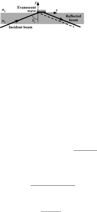
FIGURE 16.1. TIR of an incident beam of light at a refractive index interface and the generation of an evanescent wave in the less dense medium of index n1. Note that the actual reflected beam is slightly offset from the geometrically reflected light ray due to the Goos-H¨anchen effect [18].

where kt is the wavenumber. The solution with the positive exponential is physically impossible. The resultant wave therefore has an amplitude that decays exponentially with distance normal to the interface y and propagates along the direction parallel to the interface x. The intensity of the evanescent wave is proportional to the square of the transmitted electric field magnitude, and it can then be shown that this intensity

Here, Io is the intensity at the interface (i.e., y = 0), yp is the penetration depth of the evanescent wave, and λo is the wavelength of the light in vacuum.

The components of the electric field tangential to the interface must be continuous across the interface. For light polarized perpendicular to the plane of incidence (i.e., the x–y plane) with an electric field magnitude incident upon the interface of Ei , the Fresnel Equations for the amplitude transmission coefficient gives the y-component of the electric

Ei||, the Fresnel Equations give the x- and y-components of the evanescent-wave electric field at the interface as:

$

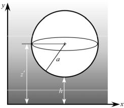
FIGURE 16.2. Sphere illuminated by an evanescent wave.

through the dense medium, only light emitted by the bottom half of the sphere facing the interface will be detected by the imaging system, and the amount of light imaged, or the brightness”“ B of the particle, will be proportional to the net power emitted by the bottom half of the sphere. It can then be shown that the image brightness of a spherical particle illuminated by an evanescent wave also decays exponentially, albeit in h, or the distance from its nearest edge to the interface, as follows:

where Bo is the brightness of the particle when it is in contact with the wall [22].

The size of such a particle imaged through a microscope objective and recorded on a CCD camera is essentially the convolution of the geometric and diffraction-limited images since a < λo in nPIV. If both these images can be approximated as Gaussian functions, this convolution is then also a Gaussian function for a spherical particle with its center at the

Here, M and NA are the magnification and numerical aperture, respectively, of the microscope objective and no is the refractive index of the immersion medium (e.g., oil) between the objective and the object.

16.3.2. Generation of Evanescent Waves

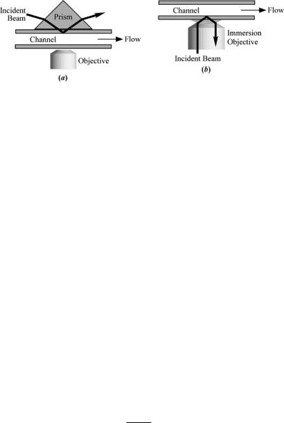
Most TIRM experiments use one of two methods to generate evanescent-wave illumination, namely the prism method based upon a prism optically coupled to the sample, or the prismless”“ method, where the evanescent wave is introduced through a high numerical aperture (NA) objective (Figure 16.3) [19]. In general, the prism method gives more flexibility in terms of optical setup, since the optics for generating the evanescent wave can be

FIGURE 16.3. Examples of TIRM configurations where the evanescent wave is generated using the (a) prism or (b) prismless”“ methods.

aligned independently of the imaging system. Two more advantages of the prism method are that it usually gives cleaner illumination, with better control over autofluorescence and/or autoluminescence, and, given the high cost of high NA microscope objectives, the prism method is usually more economical. Note that neither the prism nor the optical coupling fluid between the prism and the microchannel wall are required to have the same refractive index as the wall.

The prismless method requires a high NA immersion objective. For such an objective, Snell’s Law gives:

For water, n1 = 1.33, suggesting that NA must be well above this value; the few microscope objectives with magnifications of 60 or greater and numerical apertures of 1.45 or 1.65 are quite expensive. The major advantages of the prismless method are that this method is generally easier to implement in most microscopes, with commercial microscope vendors offering off“ -the-shelf”TIRF configurations, and that arc-lamp illumination (vs. a laser) can be used to generate the evanescent wave.

16.3.3. Brownian Diffusion Effects in nPIV

Brownian diffusion of the 100–500 nm diameter colloidal particle tracers used in microand nano-PIV can be a major source of error in both techniques. For a convective timescale τc = 1s (based upon a velocity scale of 100 µm/s and a length scale of 100 µm), the Peclet number, which compares the time required for a particle to diffuse its own radius to the convective timescale, is

Pe ≡ 6πµa3 10−3 kT τc

for a particle of radius a = 50 nm suspended in water at absolute temperature T = 300 K. In this expression, µ is the fluid viscosity and k is the Boltzmann constant. Early µPIV studies noted that the error due to Brownian diffusion imposes a practical lower limit on both the time interval between images within an image pair and the tracer particle size for a given accuracy [9]. Olsen and Adrian [25] showed that Brownian motion reduces the signal-to-noise ratio (SNR) of the cross-correlation. In steady flows, the effects of “in-plane”Brownian diffusion can be greatly reduced by temporal averaging, with the best results achieved by averaging

the cross-correlation (vs. the actual displacement) [26]. “Out-of-plane”Brownian diffusion is usually not an issue, given the out-of-plane spatial resolution of µPIV of at least 1.5 µm.

In contrast with µPIV, Brownian diffusion of nPIV tracers is hindered by the presence of the wall since particles experience increased hydrodynamic drag as they approach the wall. One of the consequences of hindered Brownian diffusion is that the diffusion coefficients are now functions of the particle distance from the wall; the hindered diffusion coefficients normal and parallel to the wall D and D|| are [27, 28]:

where h and z are the distances of the particle edge and center from the wall, respectively, and D∞ = kT /(6πµa) is the Brownian diffusion coefficient for unconfined flow [29]. Note that the expression for D is an approximation of the infinite series solution given by Goldman et al. [30].

If the tracers sample all values of h with equal probability within the y-extent illuminated by the evanescent wave, in-plane hindered Brownian diffusion can be greatly reduced for steady flows by time-averaging the nPIV data. Out-of-plane Brownian diffusion is, however, a major issue for nPIV (unlike µPIV) due to its much smaller out-of-plane spatial resolution. Diffusion normal to the wall leads to “particle mismatch, where the tracers leave (“drop out”) or enter (“drop in”) the region illuminated by the evanescent wave within the image pair, affecting the SNR of the cross-correlation.

To quantify the error due to this Brownian diffusion-induced particle mismatch, simulations were carried out of colloidal particles with initial locations generated using a Monte Carlo approach [22]. The particles were then convected over a given time interval t by a uniform velocity along x of magnitude U subject to hindered Brownian diffusion using the Langevin Equation. If the particles interact with the wall through some type of collision (instead of sticking to the wall), it was assumed that the particles interacted with the wall via perfectly elastic collisions as z /a → 1. This “wall interaction model”has a marked effect on the hindered diffusion normal to the wall, biasing the displacements due to diffusion towards lower values. Table 16.1 compares D , the diffusion coefficients predicted by Eq. (16.10) from the y-position of each particle, with D , the diffusion coefficient calculated directly from the actual particle displacement based upon the wall interaction model used here, averaged over the motion of 105 particles over 6 ms with an initial position

TABLE 16.1. Comparison of hindered Brownian diffusion coefficients for motion normal to the wall.