Biomolecular Sensing Processing and Analysis - Rashid Bashir and Steve Wereley

midplane concentration profiles for the three flow arrangements shown in Figure 14.2. In all these figures a neutral mixing species (i.e. µep = 0, thereby ignoring any electrophoretic transport) with a diffusion coefficient D = 3 × 10−10 m2/s is considered. As expected both symmetric flow fields discussed above have yielded symmetric concentration profiles as shown in Figure 14.3a and 14.3b. While mixing in the homogeneous case is purely diffusive in nature, the presence of the symmetric circulation regions, Figure 14.3b, enables enhanced mixing by two mechanisms, firstly through convective means by circulating a portion of the mixed downstream fluid to the unmixed upstream region, and secondly by forcing the bulk flow through a significantly narrower region, as shown by the convergence of the streamlines in Figure 14.2b. In Figure 14.3c the convective effects on the local species concentration is apparent from the concentration contours generated for the non-symmetrical, offset patch arrangement.

14.5. CASE STUDY II: OSCILLATING AC ELECTROOSMOTIC FLOWS IN A RECTANGULAR MICROCHANNEL

In the previous example we simulated the electroosmotically driven transport of a dilute species. As discussed in Section 14.2.1, the flow transients in such a situation need not be considered since they occur on timescales much shorter than other on-chip processes (i.e. species transport). A situation where this condition is not met is when the applied electric field is transient or time periodic. Recently the development of a series of related applications has led to enhanced interest in such time periodic electroosmotic flows or AC electroosmosis. Oddy et al. [46] for example proposed and experimentally demonstrated a series of schemes for enhanced species mixing in microfluidic devices using AC electric fields. Green et al. [28] experimentally observed peak flow velocities on the order of hundreds of micrometers per second near a set of parallel electrodes subject to two AC fields, 180◦ out of phase with each other. Brown et al. [4] and Studer et al. [57] presented microfluidic devices that incorporated arrays of non-uniformly sized embedded electrodes which, when subject to an AC field, were able to generate a bulk fluid motion. Other prominent examples include the works by Selvaganapathy et al. [55], Hughes [32] and Barrag´an [1].

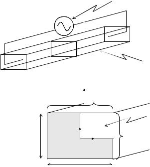
In this section we will demonstrate the modeling of an AC electroosmotic flow in a rectangular channel geometry, shown in Figure 14.4. AC electroosmotic flows are in general a good candidate for demonstrative simulation as they represent a case where the appropriate time scale (i.e. the period of oscillation) is significantly shorter than that required for the flow field to reach a steady state. For example if the AC field is applied at a frequency of 1000Hz the period of oscillation is 0.001s compared with 0.1s for the conservative case of Re = 1, discussed in Section 14.2.1. As such the transient term in Eq. (14.1a) must be considered (note that this is a simplified analysis for estimating when flow field transients should be considered, for a more detailed discussion of the relevant timescales in AC electroosmosis see Erickson and Li [15]). Further complicating matters is the work by Dutta and Beskok [12] who demonstrated that depending on the frequency and the double layer thickness there may be insufficient time for the liquid within the double layer to fully respond. As such the use of a slip condition at the edge of the double layer was shown to produce largely inaccurate results.

Thus to model this situation we consider the transient form of Eq. (14.1a), replacing the steady state , with φappsin(2π ft), where f is the frequency of oscillation. Since the flow field is uniaxial and symmetric about the center axes the computational domain is reduced

Microchannel

ζ2

Computational

Domain

lx

FIGURE 14.4. System geometry and computational domain for AC electroosmosis simulation.

to 2D in a single quadrant as shown in Figure 14.4. The double layer and applied potential fields can be decoupled, as is implied above, since the gradient of EDL field is perpendicular to the wall and the applied potential field parallel with it. The uniaxial condition implies that the derivative of the flow velocity in the lengthwise direction is zero, thus the momentum convection term in Eq. (14.1a) disappears, independent of the flow Reynolds number. Here we used the Debye-Huckel¨ linearization to determine the EDL field and net charge density, Eq. (14.9) and Eq. (14.10).

14.5.1. Flow Simulation

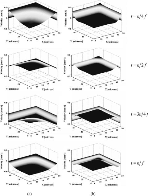
Figure 14.5 compares the time-periodic velocity profiles in the upper left hand quadrant of a 100 µm square channel for two cases (a) f = 500 hz and (b) f = 10 khz with φapp = 250 V/cm. To illustrate the essential features of the velocity profile a relatively large double layer thickness has been used, κ = 3 × 106 m−1 (corresponding to a bulk ionic concentration no = 10−6 M), and a uniform surface potential of ζ = −25 mV was selected. For a discussion on the effects of double layer thickness the reader is referred to Dutta and Beskok [12]. From Figure 14.5, it is apparent that the application of the electrical body force results in a rapid acceleration of the fluid within the double layer. In the case where the momentum diffusion time scale is much greater than the oscillation period (high f, Figure 14.2b) there is insufficient time for fluid momentum to diffuse far into the bulk flow and thus while the fluid within the double layer oscillates rapidly the bulk fluid

remains nearly stationary. At f = 500 hz there is more time for momentum diffusion from the double layer, however the bulk fluid still lags behind the flow in the double layer.

Another interesting feature of the velocity profiles shown in Figure 14.5 is the local velocity maximum observed near the corner (most clearly visible in the f = 10 khz case at t = n/4 f and t = n/2 f ). The intersection of the two walls results in a region of double layer overlap and thus an increased net charge density. This peak in the net charge density increases the ratio of the electrical body force to the viscous retardation allowing it to respond more rapidly to changes in the applied electric field and thus resulting in a local maximum in the transient electroosmotic flow velocity. Such an effect would not be observed had the slip condition approach used in Section 14.4 been implemented here.

14.6. CASE STUDY III: PRESSURE DRIVEN FLOW OVER HETEROGENEOUS SURFACES FOR ELECTROKINETIC CHARACTERIZATION

In the above two examples we limited ourselves to low Reynolds number cases where the flow field had no presumed effect on the EDL field. Here we will examine a case where such a condition is not met, specifically pressure driven slit flow over heterogeneous surfaces. Such a situation arises in a variety of electrokinetic characterization and microfluidics based applications. For example the streaming potential technique has been used to monitor the dynamic or static adsorption of proteins [13, 45, 60, 62], surface active substances [25] and other colloidal and nano-sized particles [29, 63] onto a number of surfaces. In this technique the surface’s electrokinetic properties are altered by introducing a heterogeneous region, for example due to protein adsorption, which has a different ζ-potential than the original surface. The introduction of this heterogeneous region induces a change in the surface’s average ζ -potential, which is monitored via a streaming potential measurement, and related back to the degree of surface coverage.

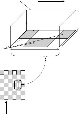
In this final example we demonstrate the simulation of pressure driven flow through a slit microchannel with an arbitrary but periodic patch-wise heterogeneous surface pattern on both the upper and lower surfaces (such that the flow field is symmetric about the midplane). Since the pattern is repeating, the computational domain is reduced to that over a single periodic cell, as shown in Figure 14.6. As mentioned above, in this example we are interested in examining the detailed flow structure and coupled effect of the flow field on the electrical double layer. As such we require a very general solution to the Poisson, Eq. (14.4), Nernst-Planck, Eq. (14.5), and Navier-Stokes, Eq. (14.1), equations in order to determine the local ionic concentration, double layer distribution and the overall flow field. Note that here in this theoretical treatment we limit ourselves to steady state flow, but we do wish to consider cases of higher Reynolds number. Thus the transient term in Eq. (14.1a) can be ignored however the higher momentum convection term should not.

14.6.1. System Geometry, Basic Assumptions and Modeling Details

In general boundary conditions on the respective equations are as described in section 2 with the exception of the inlet and outlet boundaries where periodic conditions are applied (for a general discussion on simulation in periodic domains the reader is referred to the work by Patankar et al. [50]). As mentioned above, in the absence of externally applied

Computational

Domain

Pressure Driven Flow

z

lz

Pressure

Driven

Flow

FIGURE 14.6. 3D spatially periodic computational domain for pressure driven flow through a slit microchannel with “close-packed” heterogeneous surface pattern.

electric fields the convective, streaming current components of the current conservation equation, Eq. (14.11b), is no longer dwarfed by the conduction component and thus must be considered. Additionally since we have rapid changes in the surface charge pattern, charge diffusion cannot be neglected. The highly coupled system consisting of all the general equations is difficult to solve numerically, thus several simplifying assumptions were made. Firstly it was assumed that the gradient of the induced potential field, φ, was only significant along the flow axis. Also, we assumed that Eq. (14.11b) was satisfied by applying a zero net current flux at every cross section along the flow axis, consistent with what has been done by others [7, 42]. In general we are interested in the steady state behavior of the system, thus the transient term in Eq. (14.1a) could be ignored, however we do wish to examine higher Reynolds number cases thus the convective terms should be included.

As discussed above, the resulting system of equations was solved using the finite element method. The computational domain was discretized using 27-noded 3D elements,

which were refined within the double layer region near the surface and further refined in locations where discontinuities in the surface ζ-potential were present (i.e. the boundaries between patches). In all cases periodic conditions were imposed using the technique described by S´aez and Carbonell [53].

The solution procedure here began with a semi-implicit, non-linear technique in which the ionic species concentrations and the double layer potential equations were solved for simultaneously. In general it was found that a direct solver was required as the resulting matrix was neither symmetric nor well conditioned. Once a solution was obtained the forcing term in the Navier-Stokes equations was be evaluated the flow field solved using a penalty method [30] which eliminated the pressure term from the formulation. While this reduced the number of equations that had to be solved, the resulting poorly conditioned matrix dictated the use of a direct solver over potentially faster iterative solver, such as that described in Section 14.4. Further details on the solution procedure and model verification stages are available elsewhere [19].

14.6.2. Flow Simulation

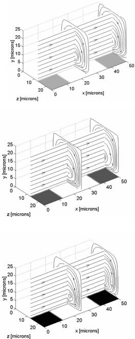
This example considers the flow over the periodic surface pattern described above with a periodic length of lx = 50 µm and width ly = 25 µm, a channel height of 50 µm (therefore ly = 25 µm in Figure 14.6). The liquid is considered as an aqueous solution of a monovalent species (physical properties of KCl from Vanysek [58] are used here) with a bulk ionic concentration of 1 × 10−5 M. Note that the selection of this reasonably low ionic concentration is equivalent to the double layer inflation techniques discussed earlier in order to bring the double layer length scale closed to that of the flow system. The Reynolds number Re = 1 and a homogeneous ζ -potential of −60 mV was selected. Figure 14.7 shows the flow streamlines for different heterogeneous ζ-potentials (a) −40 mV, (b) −20 mV and

(c) 0 mV. As can be seen the streamlines along the main flow axis remain relatively straight, as would be expected for typical pressure driven flow; however, perpendicular to the main flow axis a distinct circular flow pattern can be observed. In all cases the circulation in this plane is such that the flow near the surface is always directed from the lower ζ-potential region (in these cases the heterogeneous patch) to the higher ζ-potential region. As a result the direction of circulation is constantly changing from clockwise to counterclockwise along the x-axis as the heterogeneous patch location switches from the right to the left side. It can also be observed that the center of circulation region tends to shift towards the high ζ-potential region as the difference in the magnitude of the homogeneous and heterogeneous ζ-potential is increased. The observed flow circulation perpendicular to the pressure driven flow axis is the result of an electroosmotic body force applied to the fluid continua caused by the differences in electrostatic potential between the homogeneous surface and the heterogeneous patch [19]. In general it was found that the strength of this circulation was proportional to both Reynolds number and double layer thickness.

14.6.3. Double Layer Simulation

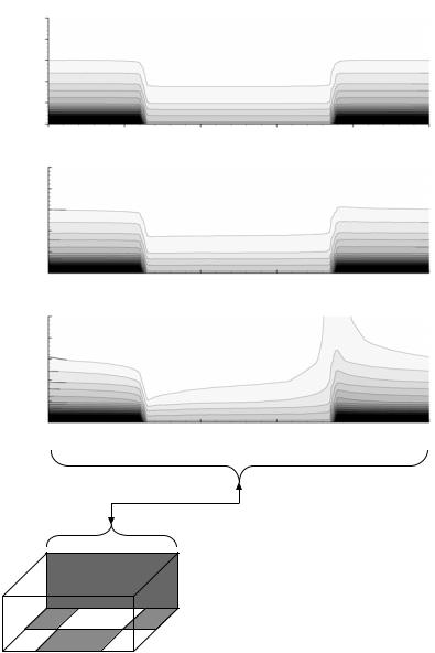
Figure 14.8 shows the influence of the flow field on the double layer distribution along the indicated plane in the computational domain at Reynolds numbers of (a) Re = 0.1,

(b) Re = 1 and (c) Re = 10 respectively. In all cases the heterogeneous ζ potential is

−40 mV and the bulk ionic concentration is 1 × 10−5 M. As can be seen the double layer field becomes significantly distorted at higher Reynolds numbers, when compared to the diffusion-dominated field at Re = 0.1 and Re = 1. The diffusion-dominated field in these cases represents a classical Poisson-Boltzmann distribution. This distortion of the double layer field is the result of a convective effect observed by Cohen and Radke [7] in their 2D numerical work and comes about as a result of an induced y-direction velocity in the transition region between the two heterogeneous surfaces. This velocity perpendicular to the surface is a result of a weaker electroviscous effect over the lower ζ potential heterogeneous patch (see Li [38] for a discussion on the electroviscous effect) and thus the velocity in the double layer is locally faster. To maintain continuity, a negative y-direction velocity is induced when flow is directed from a higher ζ-potential region (i.e. more negative) to a lower and a positive y-direction velocity is induced for the opposite case.

14.7. SUMMARY AND OUTLOOK

In this chapter we have described the relevant equations, assumptions and numerical techniques involved in performing efficient microscale flow and transport simulation for microfluidic and lab-on-chip systems. There are very few “standard” problems in such systems and thus through a series of illustrative examples we have endeavored to demonstrate the range of complexity which may be required depending on the information of interest.

In this work we have limited our discussion to flow and species transport systems. These two aspects form the fundamental basis for the operation of most Lab-on-Chip devices and cover the majority of what many researchers are interested in simulating at present. In general however they do not present a complete picture of what is required to engineer a true lab- on-chip. The majority of the developmental work in Lab-on-Chip simulation is currently directed towards either the examination of more complex flow systems, particularly those with non-uniform electrical conductivity [52], those involving thermal analysis [16], or those which couple reaction kinetics to the transport problem [17]. The eventual goal is towards the integration of all these models into a single “numerical prototyping” platform enabling the coupled simulation of microfluid dynamics, microtransport, microthermal, micromechanics, microelectronics and optics with chemical and biological thermodynamics and reaction kinetics.

REFERENCES

[1]V.M. Barrag´an and C.R. Bauz´. Electroosmosis through a cation-exchange membrane: Effect of an ac perturbation on the electroosmotic flow. J. Colloid Interface Sci., 230:359, 2000.

[2]G.K. Batchelor. An Introduction to Fluid Dynamics, Cambridge University Press, Cambridge, 2000.

[3]R.B. Bird, W.E. Stewart, and E.N. Lightfoot. Transport Phenomena, John Wiley & Sons, New York, 1960.

[4]B.D. Brown, C.G. Smith, and A.R. Rennie. Fabricating colloidal particles with photolithography and their interactions at an air-water interface. Phys. Rev. E, 63:016305, 2001.

[5]F. Bianchi, R. Ferrigno, and H.H. Girault. Finite element simulation of an electroosmotic-driven flow division at a T-junction of microscale dimensions. Anal. Chem., 72:1987, 2000.

[6]C.-H. Chen, H. Lin, S. K. Lele, and J.G. Santiago. Proceedings of ASME International Mechanical Engineering Congress. ASME, Washington IMECE2003–55007, 2003.

[7]R. Cohen and C.J. Radke. Streaming potentials of nonuniformly charged surfaces. J. Colloid Interface Sci., 141:338, 1991.

[8]A. de Mello. Plastic fantastic? Lab-on-a-Chip, 2:31N, 2002.

[9]S.K. Dertinger, D.T. Chiu, N.L. Jeon, and G.M. Whitesides. Generation of gradients having complex shapes using microfluidic networks. Anal. Chem., 73:1240, 2001.

[10]V. Dolnik, S. Liu, and S. Jovanovich. Capillary electrophoresis on microchip Electrophoresis, 21:41, 2000.

[11]D.C. Duffy, J.C. McDonald, O.J.A. Schueller, and G.M. Whitesides. Rapid prototyping of microfluidic systems in poly(dimethylsiloxane) Anal. Chem., 70:4974, 1998.

[12]P. Dutta and A. Beskok. Analytical solution of combined eloectoossmotic/pressure driven flows in twodimensional straight channels: Finite debye layer effects. Anal. Chem., 73:5097, 2001.

[13]A.V. Elgersma, R.L.J. Zsom, L. Lyklema, and W. Norde. Adsoprtion competition between albumin and monoclonal immunogammaglobulins on polystyrene lattices. Coll. Sur., 65:17. 1992.

[14]D. Erickson and D. Li. Integrated microfluidic devices. Anal. Chimica Acta, 507:11, 2004.

[15]D. Erickson and D. Li. Analysis of alternating current electroosmotic flows in a rectangular microchannel. Langmuir, 19:5421, 2003.

[16]D. Erickson, D. Sinton, and D. Li. Joule heating and heat transfer in poly(dimethylsiloxane) microfluidic systems. Lab-on-a-Chip, 3:141, 2003a.

[17]D. Erickson, D. Li, and U.J. Krull. Modeling of DNA hybridization kinetics for spatially resolved biochips. Anal. Biochem., 317:186, 2003b.

[18]D. Erickson and D. Li. Influence of surface heterogeneity on electrokinetically driven microfluidic mixing. Langmuir, 18:1883, 2002a.

[19]D. Erickson and D. Li. Microchannel flow with patchwise and periodic surface heterogeneity. Langmuir, 18:8949, 2002b.

[20]S.V. Ermakov, S.C. Jacobson, and J.M. Ramsey computer simulations of electrokinetic transport in microfabricated channel structures. Anal. Chem., 70:4494, 1998.

[21]G.J. Fiechtner and E.B. Cummings. Faceted design of channels for low-dispersion electrokinetic flows in microfluidic systems. Anal. Chem., 75:4747, 2003.

[22]D. Figeys and D. Pinto. Proteomics on a chip: Promising developments. Electrophoresis, 22:208, 2001.

[23]L.-M. Fu, R.-J. Yang, and G.-B. Lee. Analysis of geometry effects on band spreading of microchip electrophoresis. Electrophoresis, 23:602, 2002a.

[24]L.-M. Fu, R.-J. Yang, G.-B. Lee, and H.H. Liu. Electrokinetic injection techniques in microfluidic chips. Anal. Chem., 74:5084, 2002b.

[25]D.W. Fuerstenau. Streaming potential studies on quartz in solutions of aminium acetates in relation to the formation of hemimicelles at the quartz-solution interface. J. Phys. Chem., 60:981, 1956.

[26]V.K. Garg. In V.K. Garg (ed.). Applied Computational Fluid Dynamics, Marcel Dekker, New York, p. 35, 1998.

[27]S.K. Griffiths and R.H. Nilson. Band spreading in two-dimensional microchannel turns for electrokinetic species transport. Anal. Chem., 72:5473, 2000.

[28]N.G. Green, A. Ramos, A. Gonz´alez, H. Morgan, and A. Castellanos. Fluid flow induced by nonuniform ac electric fields in electrolytes on microelectrodes. I. Experimental measurements. Phys. Rev. E, 61:4011, 2000.

[29]R. Hayes, M. Bohmer,¨ and L. Fokkink. A study of silica nanoparticle adsorption using optical reflectometry and streaming potential techniques. Langmuir, 15:2865, 1999.

[30]J.C. Heinrich and D.W. Pepper. Intermediate Finite Element Method, Taylor & Francis, Philadelphia, 1999.

[31]J.D. Holladay, E.O. Jones, M. Phelps, and J. Hu. Microfuel processor for use in a miniature power supply J. Power Sources, 108:21, 2002.

[32]M.P. Hughes. Strategies for dielectrophoretic separation in laboratory-on-a-chip systems. Electrophoresis, 23:2569, 2002.

[33]R.J. Hunter. Zeta Potential in Colloid Science: Principles and Applications, Academic Press, London, 1981.

[34]B. Jung, R. Bharadwaj, and J.G. Santiago. Thousandfold signal increase using field-amplified sample stacking for on-chip electrophoresis. Electrophoresis, 24:3476, 2003.

[35]H.J. Keh and J.L. Anderson. Boundary effects on electrophoretic motion of colloidal spheres. J. Fluid Mech., 153:417, 1985.

[36]N.A. Lacher, K.E. Garrison, R.S. Martin, and S.M. Lunte. Microchip capillary electrophoresis/electrochemistry. Electrophoresis, 22:2526, 2001.