

Biomolecular Sensing Processing and Analysis - Rashid Bashir and Steve Wereley
.pdf280 |
DAVID ERICKSON AND DONGQING LI |
used in most lab-on-chip applications typically yield very thin double layers and thus this decoupling is almost always valid within a reasonable degree of error. It is important to note that there are cases of both theoretical and practical interest to microfluidics where these two components cannot be fully decoupled as will be demonstrated in Section 14.6. For the remainder of this section however we will assume that the decoupling conditions are met and return to the more general case in that section.
14.2.2. Electrical Double Layer (EDL)
An electrical double layer is a very thin region of non-zero net charge density near the interface (in this case a solid-liquid interface) and is generally the result of surface adsorption of a charged species and the resulting rearrangement of the local free ions in solution so as to maintain overall electroneutrality [39, 40]. It is the interaction of the applied/induced electric field, discussed below, with the charge in the double layer that results in the electrokinetic effects discussed here. The double layer potential field and the net charge density are related via the Poisson equation,
· (εw ε0 ψ ) + ρe = 0, |
(14.4) |
where εo and εw are the dielectric permittivity of a vacuum (εo = 8.854 × 10⁻¹² C/Vm) and the local relative dielectric permittivity (or dielectric constant) of the liquid respectively. The ionic species concentration field within the double layer is given by the Nernst-Planck conservation equation,
· |
−Di ni − Kib Ti |
ni ψ + ni v |
= 0, |
(14.5) |
|
|
|
D z e |
|
|
|
where Di and zi are the diffusion coefficient and valence of the i th species and e(e = 1.602 × 10⁻¹⁹ C), kb (kb = 1.380 × 10⁻²³ J/K) and T are the elemental charge, Boltzmann constant and temperature respectively. The two equations are coupled by the definition of the net charge density given by,
ρe = zi eni (14.6)
i
In principal the system of Eq. (14.4) through Eq. (14.6) are coupled to the flow field by the convective (3rd) term in Eq. (14.5) and as such they must, in principal, all be solved simultaneously. This results in a highly unstable system that is difficult to solve numerically. Therefore it is commonly assumed that the convective term is small and can be ignored (thereby decoupling the double layer equations from the flow field). The second major difficulty is that in principal all charged species must be accounted for in order to accurately determine the net charge density. This tends to be exceedingly difficult particularly when one wishes to examine the multispecies buffers which are commonly used in most actual Lab-on-Chip devices. Thus it is typical to implement a two species model based on the most highly concentrated ions (dominant) in the buffer solution and ignore the rest.

MICROSCALE FLOW AND TRANSPORT SIMULATION |
281 |
By far the most commonly applied boundary condition along solid walls to the Poisson equation is a fixed potential represented by the zeta potential, ζ ,
ψ = ζ |
along solid walls |
(14.7a) |
The zeta potential is a property of the solid/liquid interface and in most cases remains constant at all points in the computational domain, however there are several theoretically and practically important cases where this is not the case (Sections 14.4 and 14.6). Another possible boundary condition on Eq. (14.4) is a gradient condition related to the surface charge density, however this is not commonly used in Lab-on-Chip type applications and is often difficult to handle computationally, as the solution is no longer fixed at a point. At inflow and outflow boundaries it is common to apply a zero gradient condition,
n · ψ = 0 |
at inflow and outflow boundaries |
(14.7b) |
The proper boundary condition on the ionic species conservation equations are a zero flux condition, Eq. (14.8), which is typically applied at both solid walls and inflow and outflow boundaries,
−Di (n · ni ) − |
Di zi e |
ni (n · ψ ) + ni v = 0 at all boundaries |
(14.8) |
kb T |
This general condition is significantly less complicated than it first appears. At the solid walls v = 0 thus eliminating the convective term. At the inflow and outflow boundaries n · ψ = 0 thereby eliminating the electrophoretic (2nd) term (though not completely correct it is often common to also neglect the convective (3rd) term, as outlined above, leaving the much simpler n · ni = 0 condition).
As mentioned, the above formulation, while general, is typically very difficult to implement in most practical cases. By decoupling the potential field from the double layer field, assuming that the dielectric constant is uniform everywhere and using a model a symmetric electrolyte where both n+ and n− have the same bulk concentration of no, the system of equations above reduces to the much simpler Poisson - Boltzmann distribution which, after
linearization, yields the Debye-Huckel¨ |
approximation to the double layer field, |
|
2ψ − κ2ψ = 0 |
(14.9) |
|
where κ is the Debye-Huckel¨ parameter and is equivalent to κ = (2z2e2no/εw εokb T )1/2, which can be solved directly subject to boundary conditions Eq. (14.7a) and Eq. (14.7b) and then used to calculate the net charge density via,
|
e = − |
|
o| | |
|
|kb T |
|
ρ |
|
2n |
z |
e sinh |
z|eψ |
(14.10) |
|
|
for use in Eq. (14.1a) (details of the Poisson-Boltzmann derivation are available through a number of sources [33, 39] and will not be discussed in detail here). As mentioned
282 |
DAVID ERICKSON AND DONGQING LI |
above Eq. (14.9) and Eq. (14.10) represent the linearized version of the Poisson-Boltzmann equations and thus some error is necessarily introduced in linearizing the non-linear equation (the linearized version is only considered exact for low zeta potential (e.g., ζ < 25 mV) [33]). For most microfluidic and biochip situations, this error tends to be reasonably small and the additional computational expense and iterative solution required to solve the full non-linear equation is often not justified (see Erickson and Li [15] for an example). The major drawback of using such a formulation is that information regarding the convective and electrical effects on the double layer field and the resulting influence on the flow structure cannot be obtained.
As is described in detail in the aforementioned reference texts, the inverse of the DebyeHuckel¨ parameter (i.e. 1/κ) is representative of the double layer thickness. Depending on the value of no this thickness can vary from close to 1 µm at low ionic concentration down to a few nanometers at high ionic concentration consistent with the buffers used in most Lab-on- Chip applications. This tends to cause a variety of numerical difficulties and requires further simplification of the above formulation the details of which are outlined in Section 14.3.
14.2.3. Applied Electrical Field
The applied electric field occurs either through direct application of an external voltage (as in electroosmotic flow) or induced via an effect known as the streaming potential. A streaming potential occurs when ions from the double layer are convected along with the bulk flow, typically pressure driven, accumulating at the downstream end resulting in a potential differences between the upstream and downstream reservoirs. In either case, the potential field is most generally governed by the conservation of current condition as below,
· j = 0 |
(14.11a) |
where j is the current flux. The current flux can be obtained by summation of the flux of each individual species multiplied by the valence and elemental charge yielding,
· |
i |
zi e −Di ni − |
kb T |
ni φ + ni v |
|
= 0. |
(14.11b) |
|
|
|
Di zi e |
|
|
|
|
Though derived from it, Eq. (14.11b) is different from the Nernst-Planck equations in that here we consider the conservation or charge as opposed to the conservation of individual species. As with the Nernst-Planck equations, in many situations it is not necessary to completely solve for Eq. (14.11b). In cases of pressure driven flow where the streaming potential is of interest, the diffusive flux (1st) term can be neglected as it tends to small compared to the remaining two. A further simplification often used in such cases is to ignore the divergence operator in Eq. (14.11b), integrate the remaining flux terms over the cross sectional area, and enforce a steady state zero net current condition where the conduction current (2nd term) has equal magnitude to the convection current (3rd term). For electroosmotic or combined flow in Lab-on-Chip systems, the conduction current tends to be much larger than the other terms and, as mentioned above, the EDL region tends to be thin. Under these conditions the 1st and 3rd terms in Eq. (14.11b) can be ignored as well as
MICROSCALE FLOW AND TRANSPORT SIMULATION |
283 |
|||
the additional conduction through the double layer yielding, |
|
|||
· (λ φ) = 0 |
(14.11c) |
|||
where λ is the bulk solution conductivity and is given by |
|
|||
λ = |
Di zi2e2ni,b |
|
(14.11d) |
|
kb T |
||||
i |
|
|||
|
|
|
||
where ni,b is the bulk concentration of the i th species. In general it is the total solution conductivity that is used in microfluidic applications and thus there is typically no need to perform the summation as shown. While there are many examples of non-uniform conductivity solutions in on-chip processes [6, 16, 34] in most cases it is assumed that a uniform solution conductivity exists everywhere. In that case λ is a constant and can be removed from the above formulation leaving a simple Laplacian to describe the applied potential field.
In most cases it is proper to assume that the channel walls are perfectly insulating, thus a zero gradient boundary condition is applied,
n · φ = 0 |
at solid walls |
(14.12a) |
The most commonly and easily applied boundary condition at the inflow and outflow boundaries is a fixed potential, similar to that described by Eq. (14.12b),
φinflow = φ1 |
at inflow and outflow boundaries for fixed potential situations |
(14.12b) |
φoutflow = φ2 |
|
|
Such an approach works quite well for fundamental studies, if an entire microfluidic chip or microchannel network is to be modeled (such that the magnitude of the externally applied voltages are well defined by the experimental conditions), or if a simple system is considered (e.g. a capillary tube). If it is desired to model only a local section of a chip however, it is often non-trivial to estimate what the magnitude of the potential field is at the various inlets and outlets. In many such cases it is easier to apply a current based boundary condition, as the current can be more easily measured externally or estimated from a circuit model. In such cases the proper boundary condition is
n · φ − J /λ A at inflow and outflow boundaries for fixed current situations
(14.12c)
where J is the current and A is the channel cross sectional area. It is important to note that in order for the solution to remain bounded a fixed potential condition must be applied at a minimum of one inflow/outflow boundary (typically an outflow boundary is fixed at zero). Floating reservoirs (i.e. those where no potential is applied) are represented by a zero current condition (similar to that applied at the channel walls).

284 |
DAVID ERICKSON AND DONGQING LI |
14.2.4. Microtransport Analysis
In the previous section the general theory required for microscale flow field simulation has been outlined. In most situations however the fluid flow itself it not of primary interest so much as it is a mechanism which can be exploited to transport the various reactants or products from one site to another. On the microscale this species transport is accomplished by 3 mechanisms: diffusion, electrophoresis, and convection. In the most general case the superposition of these three mechanisms results in, analogous to Eq. (14.5), the following conservation equation
∂ci |
= · (Di ci + µep,i ci φ − ci v) + Ri |
(14.13) |
∂t |
where ci is the local concentration of the i th species, µep is the electrophoretic mobility (µep = Di zi e/ kb T ) and Ri is a bulk phase reaction term. Species transport typically occurs on timescales much longer than those for fluid flow and thus often the transient regime is of interest. A consequence of this is that Eq. (14.13) can solved after the steady state flow field has been determined, as for most dilute solutions the species transport does not globally influence the fluid flow. An important aspect of dilute species transport analysis is that in the absence of interspecies interaction (e.g. due to either bulk or surface phase reactions), the equations are not coupled and thus can be solved separately.
The reaction term in Eq. (14.13) can take many forms but for a typical reaction a rate law type relation is often assumed which, as an example, may take the form,
RC = ka,3clA cmB − kd,3cCn |
(14.14) |
where ka,3 and kd,3 are the forward and backwards reaction rate constants (the subscript 3 is used here to emphasize that these rate constants pertain to the 3D bulk region) and the superscripts l, m and n are the order of the reaction and A, B and C represent different species [3]. If the reaction were to go to effective completion, kd is often very small and could thus be ignored. In addition to multispecies bulk phase reactions, other examples where such a reaction term may be used is to account for photon induced uncaging or photobleaching of fluorescence labeled molecules.
Boundary conditions on species concentration equations are typically very dependent on the situation of interest. However, in most Lab-on-Chip applications species are transported into the region of interest from a particular inlet and transported out through an outlet (note that due to electrophoretic transport, what constitutes an inlet for species transport may well be an outlet in fluid flow), yielding boundary conditions of the form,
ci = co |
at the inlet for the ith species. |
(14.15a) |
ci = 0 |
at all other inlets |
(14.15b) |
n · ci = 0 |
at all outlets |
(14.15c) |
where co is a known concentration. The latter of boundary conditions is not ideal, as its proper application requires that the computational domain be extended sufficiently far such that the species concentration is no longer expected to exhibit large spatial variations. It

MICROSCALE FLOW AND TRANSPORT SIMULATION |
285 |
is however typically the best approximation that can be made. Boundary conditions along solid surfaces are governed by the flux of species from the bulk solution onto the solid surface and typically takes the form shown in Eq. (14.15d)
Di (n · ci ) = ∂ci,2/∂t |
at solid surfaces |
(14.15d) |
where ci,2 represents the surface concentration of the i th species and t is time. In the absence of a heterogeneous reaction or significant adsorption/sorption into the solid matrix (typically the most common case), Eq. (14.15d) reduces to a simple zero flux condition. When heterogeneous reactions or adsorption/sorption is to be considered another level of modeling (identical in principal to the above) must typically be considered for the 2D surface. For an example of such a case the reader is referred to Erickson et al. [17] who presented a model for on-chip DNA hybridization kinetics.
14.3. NUMERICAL CHALLENGES DUE TO LENGTH SCALES AND RESULTING SIMPLIFICATION
As alluded to above, numerical modeling of microscale flow, particularly electroosmotic flow, in microstructures is complicated by the simultaneous presence of three separate length scales; the channel length (mm), the channel depth or width (µm) and the double layer thickness, 1/κ (nm), which we will refer to as L1, L2 and L3 respectively. In general the amount of computational time and memory required to fully capture the complete solution on all three length scales would make such a problem nearly intractable. Since the channel length and cross sectional dimensions are required to fully define the problem (L1, L2), most computational studies have resolved this problem by either eliminating or increasing the length scale associated with the double layer thickness (L3). Bianchi et al. [5], Patankar and Hu [49] and Fu et al. [23] accomplished this by artificially inflating the double layer thickness to bring its length scale nearer that of the channel dimensions. This allowed them to solve for the EDL field, calculate the electroosmotic body force term, and incorporate it into the Navier-Stokes Equation without any further simplification. It did however not fully eliminate the third length scale and significant mesh refinement was still required near the channel wall. In a different approach Ermakov et al. [20] removed the double layer length scale (L3) from the formulation by applying a slip boundary condition to Eq. (14.1a), at the edge of the double layer, given by Eq. (14.16),
vslip = |
εw εoζ |
φ = µeo φ, |
at solid walls |
(14.16) |
η |
where µeo is the electroosmotic mobility and is a quantity commonly quoted in microfluidic studies (though geared towards electrophoresis of colloidal spheres, one of the more complete derivations of this velocity condition at the edge of the double layer is provided by Keh and Anderson [35]) and φ is evaluated at the boundary. Note that the application of boundary condition Eq. (14.12a) necessarily implies that φ is directed parallel to the boundary and that the velocity normal to the wall is identically zero as expected. Since the slip condition is applied at the edge of the double layer and not the channel wall the net
286 |
DAVID ERICKSON AND DONGQING LI |
charge density in the bulk solution is by definition negligible and thus the electroosmotic body force term in Eq. (14.1a) is eliminated. The most important consequence of the implementation of this boundary condition is that a description of the double layer field is no longer required, thus greatly simplifying the problem. While such a simplification cannot be used in cases where information regarding the flow in the double layer region is desired or required, it has been used successfully by a number of authors (Stroock et. al [56], Erickson and Li [18]) when species transport or bulk fluid motion is primary interest. An example of the implementation of this condition is provided in the following section.
Before proceeding it is worthwhile to briefly mention a few other approaches to microscale flow and transport simulation, not mentioned in the above, which may be of interest to the reader. The aforementioned paper by Fu et al. [23] provides alternative approach to the boundary conditions outlined above which they have applied to a variety of on-chip transport situations [24]. Molho et al. [43] demonstrate the use of a combined numerical simulation and optimization to study turn geometries and the resulting band spreading in microfluidic systems. Fiechtner and Cummings [21] also looked at this problem using the automated “Laplace” code, developed at Sandia National Laboratories. Though not strictly computational studies the analytical and numerical work by Griffiths and Nilson [27] and the stability analysis performed by Chen et al. [6] are also of significant interest.
14.4. CASE STUDY I: ENHANCED SPECIES MIXING USING HETEROGENEOUS PATCHES
In the preceding sections we have provided details of the equations for simulation of microfluidics and transport systems and discussed their implementation. In the following sections we will present three case studies with the objective of demonstrating the appropriate numerical implementation and approximation level depending on the information of interest. For the first of these examples we consider the enhanced species mixing in electroosmotic flow due to the presence of non-uniform electrokinetic surface properties. As discussed above, most microfluidic systems, particularly electroosmotically driven ones, are limited to the low Reynolds number regime and thus species mixing is largely diffusion dominated, as opposed to convection or turbulence dominated at higher Reynolds numbers. Consequently, mixing tends to be slow and occur over relatively long distances and times. As an example, the concentration gradient generator presented by Dertinger et al. [9] required a mixing channel length on the order of 9.25 mm for a 45 µm × 45 µm cross sectional channel or approximately 200 times the channel width to achieve nearly complete mixing. Here we use microfluidic and microtransport analysis to investigate if bulk flow circulation regions induced by heterogeneous patches can enhance species mixing.
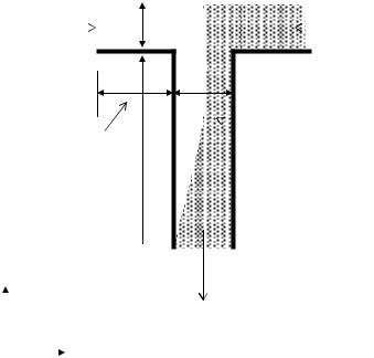
As is shown in Figure 14.1, we consider the mixing of equal portions of two buffer solutions, one of which contains a concentration, co, of a species of interest. In general the introduction of surface heterogeneity induces flow in all three coordinate directions, thus necessitating the use of a full 3D numerical simulation. In all simulations presented here a square cross section was used with the depth equaling the width of the channel, w, and the arm length, Larm. The length of the mixing channel, Lmix, was dictated by that required to obtain a uniform concentration (i.e. a fully mixed state) at the outflow boundary (thus making the application of Eq. (14.15c) at the outlet reasonable). Depending on the simulation conditions this required Lmix to be on the order of 200 times the channel width.
MICROSCALE FLOW AND TRANSPORT SIMULATION |
287 |
|
Inlet Stream 1 |
|
Inlet Stream 2 |
|
||
w
w
Larm
Mixing
Channel
Lmix
Y
Product
Stream
X
FIGURE 14.1. T-Shaped micromixer formed by the intersection of 2 microchannels, showing a schematic of the mixing/dilution process.
This is an example of a case where we are primarily interested in steady state, bulk phase fluid flow and species transport. As such we have no specific interest the double layer field and thus the electroosmotic slip condition approach, outlined in Section 14.3, is the relevant level of approximation. Therefore it was applied on all surfaces and used to simulate the hydrodynamic influence of the surface heterogeneities on the flow field and used to solve the lower Reynolds number, steady state versions of Eqs. (14.1a) and (14.1b). Additionally we assume that the transported species is dilute within a relatively highly concentrated buffer, such that the uniform conductivity assumption is met and the potential field can be determined from the Laplacian form of Eq. (14.11c) and solved subject to fixed potential conditions, Eq. (14.12b), at the inflow and outflow boundaries and insulation conditions, Eq. (14.12a), along the channel walls. The resulting species transport is modeled by the steady state, non-reactive version of Eq. (14.13).
The system of equations was solved over the computational domain via the finite element method using 27-noded triquadratic brick elements for φ, v and c and 8-noded trilinear brick elements for p. Through extensive numerical experimentation these higher order elements were found to be much more stable, especially when applied to the convection- diffusion-electrophoresis equation, than their lower order counterparts. In all cases the discretized systems of equations were solved using a quasi-minimal residual method solver and were preconditioned using an incomplete LU factorization. The advantages and disadvantages of using the finite element method (as opposed to other techniques such as control volume or finite difference) are well documented [26] and will not be discussed here other
288 |
DAVID ERICKSON AND DONGQING LI |
than to say that it is the authors’ experience that the techniques outlined above can be most easily implemented using the finite element method. Details of the finite element technique used here can be found in Heinrich and Pepper [30].
14.4.1. Flow Simulation
For the purposes of this example, we consider a test case of a channel 50 µm in width and 50 µm in depth, an applied voltage of φapp = 500 V/cm (φinlet, 1 = φinlet, 2 = φapp(Lmix + Larm), φoutlet = 0), and a mixing channel length of 15mm. We choose a homogeneous electroosmotic mobility of −4.0 × 10⁻⁸ m2/Vs, corresponding to a ζ -potential of −42 mV. An electroosmotic mobility of +4.0 × 10⁻⁸ m2/Vs was assumed for the heterogeneous patches.
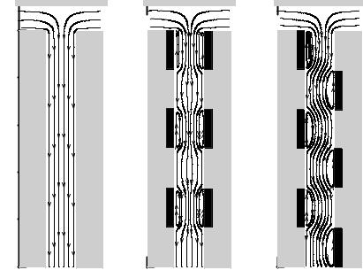
In Figure 14.2 the mid-plane flow fields near the T-intersection for the (a) homogeneous case is compared with that generated by (b) a series of 6 symmetrically distributed heterogeneous patches on the left and right channel walls and (c) a series of offset patches also located on the left and right walls respectively. For clarity the heterogeneous patches are marked as the crosshatched regions in this and all subsequent figures. As can be seen both Figures 14.2b and 14.2c do exhibit regions of local flow circulation near these heterogeneous patches, however their respective effects on the overall flow fields are dramatically
|
0 |
|
0 |
|
0 |
[microns] |
100 |
[microns] |
100 |
[microns] |
100 |
|
|
|
|||
Distance |
200 |
Distance |
200 |
Distance |
200 |
|
|
|
|||
Downstream |
300 |
Downstream |
300 |
Downstream |
300 |
|
|
|
|||
|
400 |
|
400 |
|
400 |
|
500 |
|
500 |
|
500 |
|
(a) |
|
(b) |
|
(c) |
FIGURE 14.2. Electroosmotic streamlines at the midplane of a 50 µm T-shaped micromixer for the (a) homogeneous case with ζ = −42 mV, (b) heterogeneous case with six symmetrically distributed heterogeneous patches on the left and right channel walls and (c) heterogeneous case with six offset patches on the left and right channel walls. All heterogeneous patches are represented by the crosshatched regions and have a ζ = +42 mV. The applied voltage is 500 V/cm.
MICROSCALE FLOW AND TRANSPORT SIMULATION |
289 |
different. In Figure 14.2b it is apparent that the symmetric circulation regions force the bulk flow streamlines to converge into a narrow stream through the middle of the channel. The curved streamlines shown in Figure 14.2c show the more tortuous path through which the bulk flow passes as a result of the offset, non-symmetric circulation regions.
14.4.2. Mixing Simulation
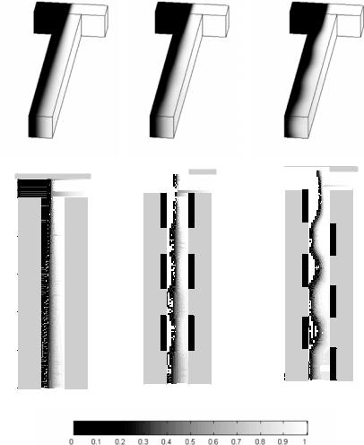
As discussed above the goal of these simulations was to examine the effect of these circulation regions on species mixing. Figure 14.3 compares both the 3D and the channel
Downstream Distance [microns]
0 |
|
0 |
|
0 |
|
|
|
||
[microns]DistanceDownstream |
|
[microns]DistanceDownstream |
|
|
100 |
100 |
100 |
||
|
|
|
||
|
|
|
|
|
200 |
|
200 |
|
200 |
|
|
|
||
|
|
|
|
|
|
|
300 |
|
300 |
300 |
|
|
|
|
|
|
|
|
|
|
|
400 |
|
400 |
400 |
|
|
|
|
|
|
|
|
|
|
|
500 |
|
500 |
500 |
|
|
|
|
|
|
|
|
(a) |
(b) |
(c) |
FIGURE 14.3. 3D species concentration contours (upper image) the midplane contours (lower image) for the 50 µm T-shaped micromixer resulting from the flow fields shown in Figure 14.2; (a) homogeneous case, (b) heterogeneous case with symmetrically distributed heterogeneous patches, and (c) heterogeneous case with offset patches. Species diffusivity is 3 × 10⁻¹⁰ m2/s and zero electrophoretic mobility is assumed.