

Biomolecular Sensing Processing and Analysis - Rashid Bashir and Steve Wereley
.pdf270 |
S.T. WERELEY AND I. WHITACRE |
|
40 |
|
|
|
|
|
|
|
|
|
|
|
|
|
|
|
0.5V |
|
35 |
|
|
|
|
|
|
1.0V |
|
|
|
|
|
|
|
2.0V |
|
|
|
|
|
|
|
|
|
|
(microns/sec) |
|
|
|
|
|
|
|
2.5V |
30 |
|
|
|
|
|
|
3.5V |
|
|
|
|
|
|
|
4.0V |
||
|
|
|
|
|
|
|
||
25 |
|
|
|
|
|
|
|
|
|
|
|
|
|
|
|
|
|
Velocity |
20 |
|
|
|
|
|
|
|
|
|
|
|
|
|
|
|
|
Axial |
15 |
|
|
|
|
|
|
|
|
|
|
|
|
|
|
|
|
Average |
10 |
|
|
|
|
|
|
|
|
|
|
|
|
|
|
|
|
|
5 |
|
|
|
|
|
|
|
|
0 |
20 |
40 |
60 |
80 |
100 |
120 |
140 |
|
0 |
Axial Position (microns)
FIGURE 13.7. Average axial velocity from PIV results for all electrode voltage cases.
Another interesting result apparent from Figure 13.7 is that initially the average particle velocity increases as the voltage increases, 0.5 volts to 2.0 volts. This phenomenon is explained by particles being displaced from the channel bottom into faster areas of the fluid flow. This biases the velocity distribution toward higher velocities, altering the shape of the cross-correlation peak to favor higher velocities even though the fluid flow is constant. For higher voltages the effect of particles being hindered by axial field gradients is compounded by particles being forced beyond the high speed central portion of the flow profile by the DEP force. It can be qualitatively confirmed that particles migrate to the top of the channel by observing particle shapes in the images from the higher voltage cases, i.e. comparing the many particle shapes found in Figure 13.2 (top) which is acquired at 0.5 volts with the single particle shape found in Figure 13.2 (bottom) which is acquired at 4.0 volts. It is confirmed that the particles are indeed at the top of the channel by moving the focal plane throughout the measurement volume.
TABLE 13.2. Curve fit parameters (V = A x + B + C sin(2 pi/D + E) for averaged axial velocities measured in microns per second.
Voltage |
A |
B |
C |
D |
E |
0.5V |
0.0326 |
16.0 |
0.869 |
42.3 |
2.83 |
1.0V |
0.0334 |
17.9 |
0.654 |
43.2 |
3.72 |
2.0V |
0.0269 |
20.6 |
0.795 |
42.1 |
3.16 |
2.5V |
0.0228 |
14.3 |
1.08 |
44.9 |
4.91 |
3.5V |
0.00800 |
11.0 |
3.50 |
39.6 |
3.95 |
4.0V |
0.00400 |
6.97 |
5.47 |
40.1 |
3.83 |
PARTICLE DYNAMICS IN A DIELECTROPHORETIC MICRODEVICE |
271 |
|
1.2 |
|
|
|
|
|
|
|
|
|
|
|
|
|
|
|
A |
|
1 |
|
|
|
|
|
|
B |
Value |
|
|
|
|
|
|
C |
|
0.8 |
|
|
|
|
|
|
|
|
Coefficient |
|
|
|
|
|
|
|
|
0.6 |
|
|
|
|
|
|
|
|
0.4 |
|
|
|
|
|
|
|
|
Normalized |
|
|
|
|
|
|
|
|
0.2 |
|
|
|
|
|
|
|
|
0 |
|
|
|
|
|
|
|
|
|
|
|
|
|
|
|
|
|
|
-0.2 |
1 |
1.5 |
2 |
2.5 |
3 |
3.5 |
4 |
|
0.5 |
Voltage ( V)
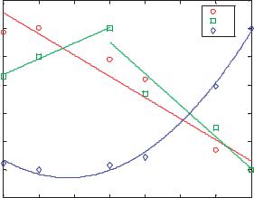
FIGURE 13.8. Curve fit parameters from (V = A x + B + C sin(2 pi/D + E) versus electrode voltage; dashed lines represent linear, piecewise linear, and parabolic curve fits for parameters A, B, and C, respectively.
The experimental results in Figure 13.7 were fit to the function
Vaxial = A · x + B + C · sin |
D + E |
(13.5) |
|
|
|
2π |
|
by minimizing the root mean squared error between the function and the experimental data. The resulting constants capture important dynamics of the particle velocity. The linear portion captures particles speeding up or slowing down over the total length of the device while the sinusoidal portion captures the dynamics of particles responding to each electrode. These results are tabulated in Table 13.2 and shown graphically in Figure 13.8. The parameters for the cases of 0.5 to volts 2.5 volts are very similar, with the exception of a gradual increase in “B”. In the two highest voltage cases the linear slope, “A” is reduced to nearly zero, and the magnitude of the sinusoidal component, “C” is greatly increased. From these results it is apparent that the particle velocities are reduced as particles travel downstream for low electrode voltages, and that the particles are dominated by a periodic trajectory for higher electrode voltages.
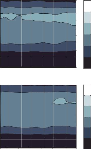
Synthetic Image Analysis The PIV images acquired from the dielectrophoretic device were analyzed a second time using the synthetic image method to extract velocity distributions at various cross-sections of the device. The analysis of the device showed a displacement distribution of roughly zero to ten pixels. This distribution was used to approximate the maximum range of velocities, and correspondingly an interrogation region with a minus five pixel integer window shift was used to center the distribution in the cross-correlation plane; centering the measurement minimizes bias errors.
From the PIV analysis it can be seen that particles move perpendicular to the electrodes or axially, so an interrogation region of 48 pixels axially by 346 pixels transversely was
272 |
S.T. WERELEY AND I. WHITACRE |
used. The effective measurement volume is the full channel depth by the imaged channel width by 53 pixels in the axial direction. A measurement was made every ten pixels in the axial direction, considerably over-sampled. The results are given in Figure 13.9, with the fluid flowing from right to left. This analysis reports the particle velocity distributions, which offer a better characterization of the flow than the conventional PIV analysis. The velocity distributions offer an additional dimension of information that is unavailable from a conventional PIV analysis.
a) |
|
|
|
|
|
|
|
0.06 |
|
35 |
|
|
|
|
|
|
|
|
30 |
|
|
|
|
|
|
0.05 |
(microns/sec) |
|
|
|
|
|
|
|
|
25 |
|
|
|
|
|
|
0.04 |
|
|
|
|
|
|
|
|
||
|
|
|
|
|
|
|
|
|
|
20 |
|
|
|
|
|
|
|
Velocity |
15 |
|
|
|
|
|
|
0.03 |
10 |
|
|
|
|
|
|
|
|
|
|
|
|
|
|
|
|
|
|
|
|
|
|
|
|
|
0.02 |
|
5 |
|
|
|
|
|
|
|
|
0 |
|
|
|
|
|
|
0.01 |
|
-5 |
|
|
|
|
|
|
|
|
20 |
40 |
60 |
80 |
100 |
120 |
140 |
0 |
|
|
Position (microns)
Probability Density (sec/micron)
b) |
|
|
|
|
|
|
0.06 |
|
|
|
|
|
|
|
|
|
|
(microns/sec)Velocity |
35 |
|
|
|
|
|
|
(sec/micron)DensityProbability |
30 |
|
|
|
|
|
0.05 |
||
|
|
|
|
|
|
|
||
|
25 |
|
|
|
|
|
|
|
|
|
|
|
|
|
|
0.04 |
|
|
20 |
|
|
|
|
|
|
|
|
15 |
|
|
|
|
|
0.03 |
|
|
10 |
|
|
|
|
|
|
|
|
|
|
|
|
|
|
0.02 |
|
|
5 |
|
|
|
|
|
|
|
|
0 |
|
|
|
|
|
0.01 |
|
|
-5 |
|
|
|
|
|
|
|
|
20 |
40 |
60 |
80 |
100 |
120 |
0 |
|
|
140 |
|
Position (microns)
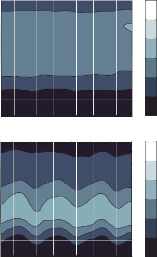
FIGURE 13.9. Probability density function for axial particle speed as a function of axial position within the DEP particle trap for electrode voltages of a) 0.5 volts, b) 1.0 volts, c) 2.0 volts, d) 2.5 volts, e) 3.5 volts and f) 4.0 volts.
PARTICLE DYNAMICS IN A DIELECTROPHORETIC MICRODEVICE
c)
|
35 |
|
|
|
|
|
|
|
30 |
|
|
|
|
|
|
(microns/sec) |
25 |
|
|
|
|
|
|
20 |
|
|
|
|
|
|
|
15 |
|
|
|
|
|
|
|
|
|
|
|
|
|
|
|
Velocity |
10 |
|
|
|
|
|
|
5 |
|
|
|
|
|
|
|
|
|
|
|
|
|
|
|
|
0 |
|
|
|
|
|
|
|
-5 |
|
|
|
|
|
|
|
20 |
40 |
60 |
80 |
100 |
120 |
140 |
Position (microns)
d)
|
35 |
|
|
|
|
|
|
|
30 |
|
|
|
|
|
|
(microns/sec) |
25 |
|
|
|
|
|
|
20 |
|
|
|
|
|
|
|
15 |
|
|
|
|
|
|
|
|
|
|
|
|
|
|
|
Velocity |
10 |
|
|
|
|
|
|
5 |
|
|
|
|
|
|
|
|
|
|
|
|
|
|
|
|
0 |
|
|
|
|
|
|
|
-5 |
|
|
|
|
|
|
|
20 |
40 |
60 |
80 |
100 |
120 |
140 |
Position (microns)
FIGURE 13.9. (Continued )
273
0. 06
0. 05 |
(sec/micron) |
|
|
||
0. 04 |
Density |
|
0. 03 |
||
Probability |
||
0. 02 |
||
|
||
0. 01 |
|
|
0 |
|
|
0. 06 |
(sec/micron) |
|
0. 05 |
||
|
||
0. 04 |
Density |
|
0. 03 |
||
0. 02 |
Probability |
|
|
0. 01
0
For the cases from 0.5 to 2.0 volts, the particle velocity distribution is as expected for flow in a slot, with the exception of a slight inclination of the contour lines that is consistent with Figure 13.7. The transition of the velocity distributions between the cases of 2.0 volts and 2.5 volts is quite dramatic. It can be seen that the bulk particle velocity is substantially reduced, while a fair number of particles still acquire high velocities. As the voltage is further increased the percentage of high speed particles is greatly reduced.
Particles travel from right to left so it can be seen from Figure 13.9 (d) that particles reach their maximum velocity faster than they slow to their minimum velocity. This is expected
274 |
S.T. WERELEY AND I. WHITACRE |
e) |
|
|
|
|
|
|
0.06 |
|
|
|
|
|
|
|
|
|
|
(microns/sec)Velocity |
35 |
|
|
|
|
|
|
(sec/micron)DensityProbability |
30 |
|
|
|
|
|
0.05 |
||
|
|
|
|
|
|
|
||
|
|
|
|
|
|
|
|
|
|
25 |
|
|
|
|
|
0.04 |
|
|
|
|
|
|
|
|
|
|
|
20 |
|
|
|
|
|
|
|
|
15 |
|
|
|
|
|
0.03 |
|
|
|
|
|
|
|
|
|
|
|
10 |
|
|
|
|
|
0.02 |
|
|
|
|
|
|
|
|
|
|
|
5 |
|
|
|
|
|
|
|
|
0 |
|
|
|
|
|
0.01 |
|
|
|
|
|
|
|
|
|
|
|
-5 |
|
|
|
|
|
0 |
|
|
20 |
40 |
60 |
80 |
100 |
120 |
|
|
|
140 |
|
Position (microns)
f ) |
|
|
|
|
|
|
0.06 |
|
|
|
|
|
|
|
|
|
35 |
|
|
|
|
|
|
|
30 |
|
|
|
|
|
0.05 |
(microns/sec) |
|
|
|
|
|
|
|
25 |
|
|
|
|
|
0.04 |
|
|
|
|
|
|
|
||
|
|
|
|
|
|
|
|
|
20 |
|
|
|
|
|
|
|
15 |
|
|
|
|
|
0.03 |
Velocity |
|
|
|
|
|
|
|
10 |
|
|
|
|
|
0.02 |
|
|
|
|
|
|
|
||
|
|
|
|
|
|
|
|
|
5 |
|
|
|
|
|
|
|
0 |
|
|
|
|
|
0.01 |
|
|
|
|
|
|
|
|
|
-5 |
|
|
|
|
|
0 |
|
|
|
|
|
100 |
|
|
|
20 |
40 |
60 |
80 |
120 |
140 |
Position (microns)
Probability Density (sec/micron)
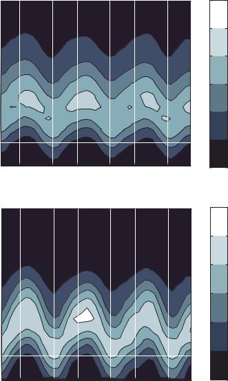
FIGURE 13.9. (Continued )
because the dielectrophoretic effect decelerates particles moving toward an electrode gap and accelerates particles moving away from a gap. The deceleration is hindered by a drag force on the particles while the acceleration is aided by the drag force.
This analysis shows that particles move fastest over the centers of the electrodes and slowest on the leading edge of the electrodes. The velocity distributions for all voltage cases
PARTICLE DYNAMICS IN A DIELECTROPHORETIC MICRODEVICE |
275 |
are plotted at the fastest and slowest positions in Figure 13.9 (e) and (f), respectively. These plots show how the velocity distributions change as voltage is increased. For the “fast” position, as voltage is increased the range of particle velocities is reduced. The range of velocities is decreased further at the “slow” position for high voltages. Another interesting observation at the “slow” position is that some particles are predicted to move in the negative axial direction. This is caused by Brownian motion of near zero velocity particles.
13.4. CONCLUSIONS
The dynamics of particles traveling through the device described in this paper are very complicated, exhibiting migration normal to the electrodes as well as trapping behavior in the plane of the electrode. Several novel µPIV interrogation techniques are applied to shed light on the particle dynamics. The results discussed in this paper provide insight into how particles respond to DEP forces. Work is in progress to generalize the results of this paper to assess whether current DEP models are sufficient for predicting how particles will respond to electrical forces.
ACKNOWLEDGEMENTS
Thanks to Professor Rashid Bashir, Haibo Li, and Rafael Gomez for providing the chip used for these experiments and also for many useful discussions about DEP. This work was partially supported by the National Science Foundation Nanoscale Science and Engineering program.
REFERENCES
[1]M. Born and E. Wolf. Principles of Optics. Oxford Press, Pergamon, 1997.
[2]E.B. Cummings. An image processing and optimal nonlinear filtering technique for PIV of microflows. Exper. Fluids, 29(Suppl.):S42–S50, 2001.
[3]J. Deval, P. Tabeling, and C.-M. Ho. A dielectrophoretic chaotic mixer. Proc. IEEE MEMS Workshop, 36–39, 2002.
[4]P.R.C. Gascoyne and J. Vykoukal. Particle separation by dielectrophoresis [Review]. Electrophoresis, 23(13):1973–1983, July 2002.
[5]N.G. Green and H. Morgan. Dielectrophoretic investigations of sub-micrometer latex spheres. J. Phys. D: Appl. Phys., 30:2626–2633, 1997.
[6]H.B. Li, Zheng, D. Akin, and R Bashir. Characterization and modeling of a micro-fluidic dielectrophoresisfilter for biological species. submitted to J. Microelectromech. Sys., 2004.
[7]C.D. Meinhart, D. Wang, and K. Turner. Measurement of AC electrokinetic flows. Biomed. Microdev., 5(2): 139–145, 2002.
[8]C.D. Meinhart, S.T. Wereley, and J.G. Santiago. A PIV algorithm for estimating time-averaged velocity fields. J. Fluids Eng., 122:809–814, 2000.
[9]R. Miles, P. Belgrader, K. Bettencourt, J. Hamilton, and S. Nasarabadi. Dielectrophoretic manipulation of particles for use in microfluidic devices. MEMS-Vol. 1, Microelectromechanical Systems (MEMS), Proceedings of the ASME International Mechanical Engineering Congress and Exposition, Nashville, TN, Nov. 14–19, 1999.
276 |
S.T. WERELEY AND I. WHITACRE |
[10]M.G. Olsen and R.J. Adrian. Out-of-focus effects on particle image visibility and correlation in microscopic particle image velocimetry. Exper. Fluids, (Suppl.):S166–S174, 2000.
[11]A. Ramos, Morgan, H., Green, N.G., and A. Castellanos. AC electrokinetics: a review of forces in microelectrode structures. J. Phys. D: Appl. Phys., 31:2338–2353, 1998.
[12]X.-B., Wang, J. Vykoukal, F. Becker, and P. Gascoyne. Separation of polystyrene microbeads using dielectrophoretic/gravitational field-flow-fractionation. Biophys. J., 74:2689–2701, 1998.
[13]S.T. Wereley, L. Gui, and C.D. Meinhart. Advanced algorithms for microscale velocimetry. AIAA J., 40(6): 1047–1055, 2002.
14
Microscale Flow and Transport Simulation for Electrokinetic and Lab-on-Chip Applications
David Erickson and Dongqing Li
Sibley School of Mechanical and Aerospace Engineering, Cornell University Ithaca, NY, 14853Department of Mechanical Engineering, Vanderbilt University Nashville, TN, 37235
14.1. INTRODUCTION
The proliferation of manufacturing techniques for building microand nano-scale fluidic devices has led to a virtual explosion in the development of microscale chemical and biological analysis systems, commonly referred to as integrated microfluidic devices or Labs-on-a-Chip [14]. Application areas into which these systems have penetrated include: DNA analysis [47], separation based detection [10, 36], drug development [59], proteomics [22], fuel processing [31] and a host of others, many of which are extensively covered in this book series. The development of these devices is a highly competitive field and as such researchers typically do not have the luxury of large amounts of time and money to build and test successive prototypes in order to optimize species delivery, reaction speed or thermal performance. Rapid prototyping techniques, such as those developed by Whitesides’ group [11, 44], and the shift towards plastics and polymers as a fabrication material of choice [8] have significantly helped to cut cost and development time once a chip design has been selected.
Computational simulation used in parallel with these rapid prototyping techniques can serve to dramatically reduce the time from concept to chip even further. Simulation allows researchers to rapidly determine how design changes will affect chip performance and thereby reduce the number of prototyping iterations. More importantly “numerical prototyping” applied at the concept stage can generally provide reasonable estimates of
278 |
DAVID ERICKSON AND DONGQING LI |
potential chip performance (e.g. rate of surface hybridization, speed of thermal cycling for PCR or separation performance in capillary electrophoresis) enabling the researcher to take a fruitful path from the beginning or conversely abandon a project that does not show promise.
In this chapter the fundamentals of microscale flow and transport simulation for Lab-on- Chip and other electrokinetic applications will be presented. The first section will provide an overview of the equations governing the analyses and numerical challenges, focusing on the aspects which separate the above from their macroscale counterparts. The physical length scales relevant to most current Lab-on-Chip devices range from 10s of nanometers to a few centimeters and thus we limit ourselves here to continuum based modeling. Following that three illustrative case studies will be presented that demonstrate the appropriate computational interrogation of these equations (i.e. assumptions and solution techniques) in order to capture all the desired information with the minimum degree of complexity.
14.2. MICROSCALE FLOW AND TRANSPORT SIMULATION
14.2.1. Microscale Flow Analysis
On the microscale fluid flow can be accomplished by several means, the most common of which are traditional pressure driven flow and electroosmotic flow [33, 41]. Another mechanism of recent interest is magnetohydrodynamic flow (in which the interaction of a magnetic field and electric field induces a Lorenz force and thereby fluid transport) [37] has many advantages however is beyond the scope of what will be covered here. In either of the two former cases fluid motion is governed by the momentum Eq. (14.1a) and continuity equations Eq. (14.1b) shown below,
ρ |
∂v |
+ v · v |
= − p + η 2v − ρe , |
(14.1a) |
|
∂t |
|
||||
|
|
|
|
· v = 0 |
(14.1b) |
where v, t, p, η , and ρ are velocity, time, pressure, viscosity and density respectively. Inherent in Eqs. (14.1) are assumptions of incompressibility and constant viscosity and thus they are effectively limited to the description of constant temperature liquid flows. While this is somewhat restrictive, particularly considering the importance of Ohmic heating in polymeric microfluidic systems [16], the approximation is usually reasonably good in high thermal conductivity chips (e.g. glass or silicon) or for pressure driven flows. The final term in Eq. (14.1a) represents the electrokinetic body force and is equivalent to the product of the net charge density in the double layer, ρe , multiplied by the gradient of the total electric field strength, . In general, the relatively small channel dimensions and flow velocities, typical of microfluidic and biochip applications, limit microscale liquid flows to small Reynolds numbers (Re = ρ Lvo/η where L is a length scale and vo the average velocity). A typical flow velocity of 1mm/s in a channel with a 100 µm hydraulic diameter yields a Reynolds number on the order of 0.1. As a result the transient and convective terms (those on the left-hand side of Eq. (14.1a)) tend to be negligibly small and thus are typically ignored in order to simplify the formulation. In the majority of cases this assumption is quite good
MICROSCALE FLOW AND TRANSPORT SIMULATION |
279 |
however it does have some consequences. The most important of which is that the lack of a transient term necessarily implies that the flow field reaches a steady state instantaneously. To quantify this, let’s consider the timescale used in the above definition of the Reynolds number, L/vo, which for the above example yields 0.1s. As such if the other quantities of interest (e.g. species transport and surface reactions) which are being studied occur on timescales greater than 0.1s, which most do, the assumption that the flow field reaches an instantaneous steady state is valid. In sections 5 and 6 of this chapter we will provide examples of higher Reynolds number and transient situations where the above assumptions are not met.
Along solid walls, the general proper boundary conditions on Eq. (14.1a) is a no slip condition as described by Eq. (14.2a),
v = 0. |
at solid walls |
(14.2a) |
Inflow and outflow boundary conditions are generally more involved, depending on the situation. When pure electroosmotic flow is to be considered (that is to say there is no externally applied pressure, which does not preclude the possibility of internally induced pressure gradients), a simple zero gradient boundary condition normal to the inlet, Eq (14.2b)
n · v = 0 |
at inflow boundaries in pure EO flow and outflow boundaries (14.2b) |
where n is the unit normal to the surface, and a no flow boundary condition parallel with the inlet can be applied. When an external pressure driven flow component is present the inlet boundary condition is typically represented by the summation of a parabolic velocity profile (accounting for the pressure driven component) and a plug flow profile (accounting for the electroosmotic component) applied at the inlet boundaries. The form of the pressure driven flow component of the boundary condition varies significantly based on the inlet geometry and thus the reader is referred to standard fluid mechanics references such as Panton [48], White [61] or Batchelor [2] for exact forms. Another possibility is to apply a pressure based body force to the fluid continuum, as will be done in Section 14.6. This is particularly useful when the inlet/outlet boundary conditions are not apparent (e.g. periodic cases) but it does require prior knowledge of the pressure distribution and is thus not practical in most cases. The proper outflow boundary condition for all these cases is a zero gradient in the normal direction and no flow tangential to the boundary, similar to that for the inlet in the pure EO flow case, Eq. (14.2b). The above boundary conditions are very specific to confined liquid flows and are not sufficient for all systems (e.g. those involving free surfaces and capillarity). For a more general formulation the reader is referred to Reddy and Gartling [51].
As is apparent from Eq. (14.1a) evaluation of the momentum equation requires a description of the net charge density, ρe , and the total electrical field, . The total electric field is commonly split into two components: the electrical double layer field (EDL), ψ , and the applied electric field, φ, as per Eq. (14.3) below,
= φ + ψ. |
(14.3) |
The decoupling of these two terms is contingent on a number of assumptions that are well described in the often-quoted work by Saville [54]. The relatively high ionic strength buffers