Biomolecular Sensing Processing and Analysis - Rashid Bashir and Steve Wereley

FIGURE 16.4. Representative (a) artificial and (b) experimental particle tracer images.

z /a = [1 : ]. For all values of , D < D , and, as expected, the discrepancy between the two values decreases as increases. This result demonstrates that experimental measurements of hindered Brownian diffusion normal to the wall where the particle interacts with the wall via some type of elastic collision will underestimate the Brownian diffusion coefficient and that any such measurement will be very sensitive to particle-wall interaction effects due, for example, to surface charge or roughness.

An artificial image pair is then generated based upon the initial locations of these particle tracers and their locations after a time interval t . The particle images are modeled as a Gaussian intensity distribution with an effective diameter given by Equation (16.8) and a peak grayscale value calculated using Equation (16.7). The particle number density, image shape and image background noise characteristics are adjusted so that they match those for a typical experimental nPIV image following the guidelines suggested by Westerweel [31]. Figure 16.4 shows representative artificial and experimental images.

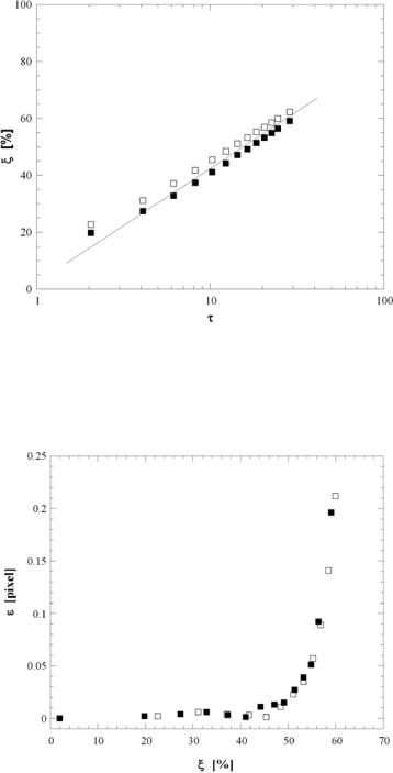
Datasets consisting of 5000 such artificial image pairs were processed using FFT–based cross-correlation (cf. Sec. 16.4.1) and a Gaussian (correlation) peak-finding algorithm using a Gaussian surface fit over at least 11 neighboring points for 118 × 98 pixel interrogation windows with 50% overlap. These relatively large interrogation windows were chosen to match experimental data (cf. Section 16.4); in all cases, at least 30 particle images were present in each window. Figure 16.5 shows the fraction of mismatched particles (as a percentage of the total number of particles) within an image pair ξ as a function of the time interval within the image pair normalized by the time required for a particle to diffuse its radius due to Brownian motion τ = t /(a2/D∞). The results averaged over 5000 image pairs for both unconfined ( ) and hindered ( ) Brownian diffusion show that the percentage of mismatched particles increases logarithmically with τ for τ > 5, and that mismatch is reduced by about 5% for hindered diffusion.

Figure 16.6 shows the displacement error ε between the results obtained by processing an artificial image pair with the actual displacement of U ( t ) as a function of particle mismatch averaged over 5000 image pairs. This error is well below the typical minimum accuracy of cross-correlation-based PIV results of about 0.05 pixels [32] and essentially constant for ξ < 45%. Results for both unconfined ( ) and hindered ( ) Brownian diffusion show a sharp increase in the displacement error once ξ exceeds 55%. This rapid increase in ε for larger values of ξ is due to a decrease in SNR of the cross-correlation peak from both a decrease in the height and an increase in the width of the peak [22]. Note that for a minimum of 30 particles per interrogation window, ξ = 55% implies that there are at least 13 “matched”particles in each image pair, more than twice the minimum value of

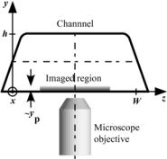
FIGURE 16.7. Definition sketch of channel cross-section and summary of channel dimensions. Here, x is the flow direction, y is the direction normal to the wall (i.e., along the optical axis) and z is along the wall normal to x.

16.4. NANO-PIV RESULTS IN ELECTROOSMOTIC FLOW

16.4.1. Experimental Details

Electroosmotic flow (EOF) of dilute aqueous solutions of the weak base sodium tetraborate (Na2B4O7), or borax, at molar concentrations C = 0.19–36 mM was studied in rectangular fused silica microchannels with cross-sectional dimensions h × W (Figure 16.7) [34]. At these concentrations, the salt dissociates in aqueous solution to give anion and cation species with a valence of unity:

Na2B4O7 + 7H2O 2Na+ + 2B(OH)3 + 2B(OH)4−

and molar concentration of the ith ionic species, respectively).

The microchannels were fabricated using chemical wet etching to produce an open trapezoidal channel, which was then sealed with a cover slip. The region of the microchannel imaged in these experiments was at least 360h downstream of any bends or intersections to ensure fully-developed flow, next to the cover slip at the bottom of the channel to minimize surface roughness and in the center of the channel to ensure uniform flow along the z-direction.

The working fluid was seeded with 100 nm diameter fluorescent polystyrene spheres (Estapor XC, Bangs Laboratories, Inc.) at volume fractions of 0.07–0.1%. The spheres have excitation and emission maxima at 480 nm and 520 nm, respectively, and a density ρ = 1.05 g/cm3. The microchannel was allowed to sit for several minutes after filling the reservoirs at both ends of the channel with the working fluid to ensure that any Poiseuille flow was eliminated before imposing an electric field using platinum electrodes in the reservoirs.

The evanescent-wave illumination was generated using the prism method (cf. Section 16.3.2) from a continuous argon-ion laser (Coherent Innova 90) beam at 488 nm with an output power of approximately 0.1 W. The beam is refracted through an isosceles

right-angle triangle prism and undergoes TIR with an angle of incidence θ ≈ 70◦ at the interface between the fused silica cover slip with a refractive index n2 = 1.46 and the water with refractive index n1 = 1.33. The penetration depth of the evanescent wave yp, which determines the out-of-plane spatial resolution of these measurements, is 90–110 nm.

The fluorescent particle tracers are imaged with an inverted epi-fluorescent microscope (Leica DMIRE2) equipped with a 63 × 0.5 objective (Leica PL Fluotar L) and a dichroic beamsplitter cube (Leica I3) to ensure that only the longer-wavelength fluorescence from the particles is imaged as 100 row × 653 column images (nominal dimensions) on a CCD camera with on-chip gain (Photometrics Cascade 650) at typical framing rates of 160 Hz with 1 ms exposure.

In-house software, implemented in MATLAB version 6.5, was used to calculate flow velocities from the particle images. This processing software uses a combined correlationbased interrogation and tracking algorithm [35] to analyze an interrogation window from the first (i.e., earlier) image within the pair with dimensions (X, Z) and a larger interrogation window from the second image with dimensions of (X + 2 , Z + 2 ). The interrogation windows are cross-correlated using an FFT-based algorithm that can be applied to windows of arbitrary dimensions. The overlap between adjacent windows was 50%, and no window shift was used since the displacement in all cases was 5 pixels or less. In processing these data, the window dimensions varied with dataset, with X = 120−200 pixels, Z = 58−88 pixels and = 10−16 pixels. Note that typical window dimension of 120 × 80 pixels (x × z) corresponding to an in-plane spatial resolution of 18 × 13 µm, with 50% overlap, gives 18 particle displacement vectors for each image. The range of window sizes were chosen to ensure that the number of particle images in each window is at least 20 to ensure a cross-correlation peak with a good signal to noise ratio, even with significant particle mismatch between two successive exposures due to Brownian diffusion normal to the wall. Cross-correlation averaging [26] or “single-pixel interrogation”[36], originally used to improve the spatial resolution of µPIV data, can also be used to improve the spatial resolution of nPIV data. Although not shown here, cross-correlation averaging of a subset of these images with windows as small as 16 × 10 pixels (x × z), corresponding to an in-plane spatial resolution of 2.5 × 1.5 µm, give average velocity results within 2% of those reported here.

16.4.2. Results and Discussion

The EOF studied here is essentially uniform normal to the wall, since the electric double layer is very thin compared with yp, with a Debye length λ < 9 nm. Figure 16.8 shows a typical raw particle image and the nPIV result obtained by averaging velocity data

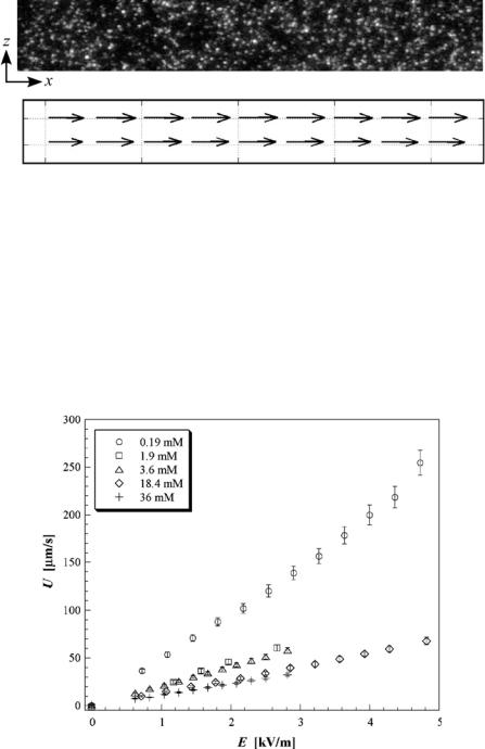
FIGURE 16.8. Representative image of particle tracers over a 110 × 16 µm (x × z) field of view [top] and corresponding nPIV result [bottom] averaged over 999 image pairs. The velocity vectors represent an average velocity U = 17.6 µm/s.

obtained over 1000 such consecutive images (= 999 image pairs) for C = 3.6 mM and E = 1.0 kV/m. The measured velocity field verifies that the flow is essentially uniform over this x–z plane.

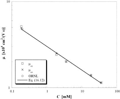
The nPIV results were therefore spatially and temporally averaged to obtain the bulk flow velocity U. Figure 16.9 shows U as a function of the external electric field E for various Na2B4O7 concentrations C. The average velocity is a linear function of the driving electric field, corresponding to constant mobility. The error bars represent conservative

FIGURE 16.9. Graph of average velocity U as a function of external electric field E for C = 0.19 − 36 mM sodium tetraborate buffer.

95% confidence intervals; these error estimates include both the uncertainty in determining particle displacement in each set of images and other experimental uncertainties associated with converting this displacement into actual velocities, such as the estimated physical dimension of one pixel in each image and the CCD camera framing rate.

As discussed in Section 16.3.3, Brownian diffusion of the 100 nm tracers can be a significant issue in nPIV data. Errors due to out-of-plane Brownian diffusion can be estimated using the results from the previous Section. For a time interval between images within the image pair t = 6.5 ms, τ = 13.3, corresponding in Figure 16.5 to a fraction of mismatched particles ξ = 45%. The results shown in Figure 16.6 suggest that the displacement error due to hindered Brownian diffusion for this level of particle mismatch is negligible.

In-plane Brownian diffusion can be estimated using calculations similar to those used to generate Table 16.1 [22]. A tracer with an initial position z /a ≤ 3 has a mean diffusion coefficient for motion parallel to the wall D||/D∞ = 0.774 averaged over 105 particles; the rms Brownian displacement parallel to the wall for a particle using this value is then x|| ≈ 220 nm, corresponding to a displacement of about one pixel, vs. the maximum displacement due to the flow of three pixels, in these experiments. Errors due to in-plane Brownian diffusion can be greatly reduced by averaging the flowfield for this steady flow over time. A typical value for the standard deviation for a single velocity vector at a given spatial location over 999 realizationswhich— should give an estimate of the in-plane Brownian diffusion averaged over all the tracer particles within the interrogation window—is6%. After temporal averaging, this standard deviation in turn accounts for about 2% of the 95% confidence intervals given in Figure 16.9. Errors associated with the imaging system (due, for example, to errors in determining the magnification of the images and the limiting spatial resolution of the CCD camera) are therefore much more significant sources of error in these experimental results.

To validate the nPIV data, the mobility µex was calculated using linear regression from the results of Figure 16.9 and compared with the electroosmotic mobility µeo predicted by the asymptotic model of Conlisk et al. [37].

In this equation, εe and µ are the electrical permittivity and absolute viscosity, respectively, of the fluid, φo ≡ RT /F is the characteristic scale for the potential formed from R the universal ideal gas constant, T the fluid absolute temperature and F Faraday’s constant, and (g0, f 0) are the wall mole fractions of the cationic and anionic species, respectively. As shown in Figure 16.10, the experimental and model values for mobility agree within 4.5% over a 200-fold change in molar concentration, suggesting that the particle tracers follow the flow with good fidelity over this range of electric fields. The mobility values are also compared with a single independent measurement using neutral fluorescent molecular tracers for C = 0.2 mM [38]. These independently obtained analytical and experimental results suggest that particle slip with respect to the fluid due to electrophoresis has a negligible effect on mobility for the EOF cases studied here. Furthermore, the mobility obtained from the nPIV data appears to be unaffected by tracer particle properties such as size and charge.

FIGURE 16.10. Log-log plot of electroosmotic mobility values as a function of C.

Finally, these results suggest that the mobility µ has a novel power-law scaling with concentration:

Note that this scaling cannot be directly derived from the analysis because of the iterative method used to derive (g0, f 0).

16.5. SUMMARY

Over the last three years, nano-particle image velocimetry—based upon tracking the motion of colloidal fluorescent particles illuminated by evanescent waveshas— been developed as a new method for measuring near-wall velocity fields with submicron spatial resolution. Initial results from this novel technique have been validated for steady fullydeveloped electroosmotic flows in microchannels, and suggest a novel scaling of electroosmotic mobility with electrolyte concentration.

Nano-PIV can measure velocities averaged over the first 100 nm based upon penetration depth next to the wall with an out-of-plane spatial resolution of 100 nm based upon

tracer particle diameter. In comparison, the near-wall capability of µPIV is about 900 nm based upon interrogation window size and its out-of-plane spatial resolution based upon depth of field is at least 1.5 µm. The method therefore represents about an order of magnitude improvement in near-wall access and out-of-plane spatial resolution over current microfluidic diagnostic techniques. The in-plane spatial resolution of these nPIV data of 18 µm ×13µm obtained here without cross-correlation averaging is significantly larger than that of the best reported µPIV measurements using cross-correlation averaging. Nevertheless, initial results using cross-correlation averaging of nPIV data show that the minimum in-plane spatial resolution of nPIV should be comparable to that for µPIV, namely 1–2 µm.

Brownian diffusion is potentially a significant source of error in nPIV, given typical Peclet numbers for the tracers used in this technique of O(10−3). Results from artificial and experimental images suggest, however, that hindered Brownian diffusionand— more specifically, particle mismatch within the image pair due to Brownian diffusionhas— relatively little impact on the accuracy of nPIV data for the steady uniform flows studied here provided that the interrogation window size is chosen to ensure enough (here, at least 11) matched tracers within an image pair.

These initial results demonstrate the potential of this technique. In terms of extending nPIV, the exponential decay of particle image intensity with distance from the wall given by Equation (16.3) suggests that it may be possible, for tracer images with sufficient contrast and tracers with consistent fluorescence intensity, to obtain not just the x- and z-positions of the particles, but also their y-position. If so, it should be possible to measure all three velocity components using nPIV without any additional imaging equipment. Particle tracking studies are already underway to measure hindered Brownian diffusion normal to the wall using this concept [39].

Finally, issues associated with particle tracers such as Brownian diffusion and, for EOF, electrophoresis, may be avoided altogether by using molecular tracers illuminated by evanescent waves to obtain near-wall velocimetry measurements. Current intensified CCD technology may not yet be sufficient for nanoscale MTV, given that the quantum efficiency of molecular tracers such as phosphorescent supramolecules is 3.5% [11], more than an order of magnitude lower than that of the fluorophores used in nPIV tracers of at least 90%. Nevertheless, Pit et al. [8] have already used a related technique, fluorescence recovery after photobleaching, with evanescent waves at a single point to show evidence of slip in hexadecane. The rapid development of single-photon and molecule imaging technology suggests that molecular tracers illuminated by evanescent waves will ultimately be the most accurate method for measuring near-wall velocity fields and studying interfacial phenomena such as apparent slip at the submicron scale.

ACKNOWLEDGEMENTS

This work would not have been possible without the contributions of Dr. Reza Sadr, Haifeng Li and Claudia M. Zettner in my group at Georgia Tech. We also wish to thank Dr. Terry Conlisk and Zhi Zheng at Ohio State University and Dr. Mike Ramsey and J.-P. Alarie at Oak Ridge National Laboratories for sharing their results and numerous suggestions.

REFERENCES

[1]Supported by DARPA DSO (F30602-00-2-0613) and NSF (CMS-9977314).

[2]G.W.Woodruff School of Mechanical Engineering; Georgia Institute of Technology; Atlanta,GA30332–0405 USA E-mail: minami.yoda@me.gatech.edu.

[3]S. Granick, Y. Zhu, and H. Lee. Nat. Mat., 2:221, 2003.

[4]P.G. De Gennes. Langmuir, 18:3413, 2002.

[5]P. Attard. Advan. Coll. Int. Sci., 104:75, 2003.

[6]O.I. Vinogradova. Int. J. Min. Proc., 56:31, 1999.

[7]D.C. Tretheway and C.D. Meinhart. Phys. Fluids, 14:L9, 2002.

[8]R. Pit, H. Hervet, and L. L´eger. Phys. Rev. Lett., 85:980, 2000.

[9]J.G. Santiago, S.T. Wereley, C.D. Meinhart, D.J. Beebe, and R.J. Adrian. Exp. Fluids, 25:316, 1998.

[10]W.R. Lempert, K. Magee, P. Ronney, K.R. Gee, and R.P. Haughland. Exp. Fluids, 18:249, 1995.

[11]C.P. Gendrich, M.M. Koochesfahani, and D.G. Nocera. Exp. Fluids, 23:361, 1997.

[12]P.H. Paul, M.G. Garguilo, and D.J. Rakestraw. Anal. Chem., 70:2459, 1998.

[13]D. Sinton and D. Li. Coll. Surf. A: Physicochem. Eng. Asp., 222:273, 2003.

[14]C. Lum and M. Koochesfahani. Bull. Am. Phys. Soc., 48(10):58, 2003.

[15]E. Bonaccurso, M. Kappl, and H.-J. Butt. Phys. Rev. Lett., 88:076103, 2002.

[16]C.M. Zettner and M. Yoda. Exp. Fluids, 34:115, 2003.

[17]E. Hecht. Optics (3rd Ed.), Addison-Wesley, Reading, p. 124, 1998.

[18]H.K.V. Lotsch. Optik 32:189, 1970.

[19]D. Axelrod, E.H. Hellen, and R.M. Fulbright. In J.R. Lakowicz (ed.), Topics in Fluorescence Spectroscopy, Vol. 3: Biochemical Applications. Plenum Press, New York, p. 289, 1992.

[20]D. Axelrod, T.P. Burghardt, and N.L. Thompson. Ann. Rev. Biophys. Bioeng., 13:247, 1984.

[21]D.C. Prieve and N.A. Frej. Langmuir, 6:396, 1990.

[22]R. Sadr, H. Li, and M. Yoda. Exp. Fluids, 38:90, 2005.

[23]R.J. Adrian. Ann. Rev. Fluid Mech., 23:261, 1991.

[24]C.D. Meinhart and S.T. Wereley. Meas. Sci. Technol., 14:1047, 2003.

[25]M.G. Olsen and R.J. Adrian. Opt. Laser Technol., 32:621, 2000.

[26]C.D. Meinhart, S.T. Wereley, and J.G. Santiago. J. Fluids Eng., 122:285, 2000.

[27]M.A. Bevan and D.C. Prieve. J. Chem. Phys., 113:1228, 2000.

[28]H. Fax´en. Ann. Phys., 4(68):89, 1922.

[29]A. Einstein. Ann. Phys., 17:549, 1905.

[30]A.J. Goldman, R.G. Cox, and H. Brenner. Chem. Eng. Sci., 22:637, 1967.

[31]J. Westerweel. Exp. Fluids, 29:S3, 2000.

[32]M. Raffel, C. Willert, and J. Kompenhans. Particle Image Velocimetry: A Practical Guide, Springer, Berlin, p. 129, 1998.

[33]R.D. Keane and R.J. Adrian. Appl. Sci. Res., 49:191, 1992.

[34]R. Sadr, M. Yoda, Z. Zheng, and A.T. Conlisk. J. Fluid Mech., 506:357, 2004.

[35]D.F. Liang, C.B. Jiang, and Y.L. Li. Exp. Fluids, 33:684, 2002.

[36]J. Westerweel, P.F. Gelhoed, and R. Lindken. Exp. Fluids, 37:375, 2004.

[37]A.T. Conlisk, J. McFerran, Z. Zheng, and D.J. Hansford. Anal. Chem., 74:2139, 2002.

[38]J.M. Ramsey, J.P. Alarie, S.C. Jacobson, and N.J. Peterson. In Y. Baba, S. Shoji, and A.J. van den Berg (eds.), Micro Total Analysis Systems 2002, Kluwer Academic Publishers, Dordrecht, p. 314, 2002.

[39]K.D. Kihm, A. Banerjee, C.K. Choi, and T. Takagi. Exp. Fluids, 37:811, 2004.

17

Optical MEMS-Based Sensor Development with Applications to Microfluidics

D. Fourguette , E. Arik , and D. Wilson#

VioSense Corporation, 36 S. Chester Ave., Pasadena, CA 91106

#Jet Propulsion Laboratory, 4800 Oak Grove Drive, Pasadena, CA 91109

17.1. INTRODUCTION

Despite challenges associated with development and fabrication, meso-scale and MEMS devices offer many advantages such as small size and lighter weight for space applications, higher reliability, smaller and better controlled sampling volumes in particular for biological diagnostics. Traditional optical diagnostics have been used to determine parameters such as velocity, concentration, particle size and temperature in laboratory-scale and full scale flow systems over the past three decades. A great deal of efforts has been invested in these diagnostics techniques, but the size of MEMS prohibits the use of these traditional diagnostics. Spatial resolution, vibrations, and optical accessibility make traditional optical setups difficult to use for microfluidics.

Recent progress in the design and fabrication of optical MEMS and beam-shaping diffractive optical elements has enabled the development of meso-scale and microsensors whose size is comparable to the scales encountered in microfluidics applications [14]. Moreover, optical MEMS can be integrated into microfluidic devices during fabrication and as such, are also suitable for on-board process monitoring.