Biomolecular Sensing Processing and Analysis - Rashid Bashir and Steve Wereley

[37]A.V. Lemoff and A.P. Lee. An AC magnetohydrodynamic micropump. Sens. Actu. B, 63:178, 2000.

[38]D. Li. Electro-viscous effects on pressure-driven liquid flow in microchannels. Coll. Surf. A, 195:35, 2001.

[39]J. Lyklema. Fundamentals of Interface and Colloid Science, Vol. 1: Fundamentals, Academic Press, London, 1991.

[40]J. Lyklema. Fundamentals of Interface and Colloid Science, Vol. 2: Solid-Liquid Interfaces, Academic Press, London, 1995.

[41]J. Masliyah. Electrokinetic Transport Phenomena. Alberta Oil Sands Technology and Research Authority, Edmonton, 1994a.

[42]J. Masliyah. Salt rejection in a sinusoidal capillary tube. J. Coll. Int Sci., 166:383, 1994b.

[43]J.I. Molho, A.E. Herr, B.P. Mosier, J.G. Santiago, T.W. Kenny, R.A. Brennen, G.B. Gordon, and B. Mohammadi. Optimization of turn geometries for microchip electrophoresis. Anal. Chem., 73:1350, 2001.

[44]J.M.K. Ng, I. Gitlin, A.D. Stroock, and G.M. Whitesides. Components for integrated poly(dimethylsiloxane) microfluidic systems. Electrophoresis, 23:3461, 2002.

[45]W. Norde and E. Rouwendal. Streaming potential measurements as a tool to study protein adsorption-kinetics.

J. Coll. Int. Sci., 139:169, 1990.

[46]M.H. Oddy, J.G. Santiago, and J.C. Mikkelsen. Electrokinetic instability micromixing. Anal. Chem., 73:5822, 2001.

[47]B.M. Paegel, R.G. Blazej, and R.A. Mathies. Microfluidic devices for DNA sequencing: Sample preparation and electrophoretic analysis. Curr. Opin. Biotechnol., 14:42, 2003.

[48]R. Panton. Incompressible Flow, John Wiley & Sons, New York, 1996.

[49]N.A. Patankar and H.H. Hu. Numerical simulation of electroosmotic flow. Anal. Chem., 70:1870, 1998.

[50]S. Patankar, C. Liu, and E. Sparrow. Fully developed flow and heat-transfer in ducts having streamwiseperiodic variations of cross-sectional area. J. Heat Trans., 99:180, 1977.

[51]J.N. Reddy and D.K. Gartling. The Finite Element Method in Heat Transfer and Fluid Dynamics, CRC Press, Boca Raton, 2001.

[52]L. Ren and D. Li. Electrokinetic sample transport in a microchannel with spatial electrical conductivity gradients J. Colloid Intefrace Sci., 294:482, 2003.

[53]A. S´aez and R. Carbonell. On the performance of quadrilateral finite-elements in the solution to the stokes equations in periodic structures. Int. J. Numer. Meth. Fluids, 5:601, 1985.

[54]D.A. Saville. Electrokinetic effects with small particles. Ann. Rev. Fluid Mech., 9:321, 1977.

[55]P. Selvaganapathy, Y.-S.L. Ki, P. Renaud, and C.H. Mastrangelo. Bubble-free electrokinetic pumping. J. Microelectromech. Syst., 11:448, 2002.

[56]A.D. Stroock, M. Weck, D.T. Chiu, W.T.S. Huck, P.J.A. Kenis, R.F. Ismagilov, and G.M. Whitesides. Patterning electro-osmotic flow with patterned surface charge. Phys. Rev. Lett., 84:3314, 2000.

[57]V. Studer, A. P´epin, Y. Chen, and A. Ajdari. Fabrication of microfluidic devices for AC electrokinetic fluid pumping. Microelect. Eng., 61:915, 2002.

[58]P. Vanysek. In D.R. Lide (ed.). CRC Handbook of Chemistry and Physics, CRC Press, 2001.

[59]B.H. Weigl, R.L. Bardell, and C.R. Cabrera. Lab-on-a-chip for drug development. Advan. Drug Del. Rev., 55:349, 2003.

[60]C. Werner and H.J. Jacobasch. Surface characterization of hemodialysis membranes based on electrokinetic measurements. Macromol. Symp., 103:43, 1996.

[61]F.M White. Fluid Mechanics, McGraw-Hill, New York, 1994.

[62]M. Zembala and P. D´ejardin. Streaming potential measurements related to fibrinogen adsorption onto silica capillaries. Coll. Surf. B, 3:119, 1994.

[63]M. Zembala and Z. Adamczyk. Measurements of streaming potential for mica covered by colloid particles. Langmuir, 16:1593, 2000.

15

Modeling Electroosmotic Flow

in Nanochannels

A.T. Conlisk and Sherwin Singer†

Department of Mechanical Engineering, The Ohio State University, Columbus, Ohio 43202

† The Department of Chemistry, The Ohio State University, Columbus, Ohio 43210-1107

15.1. INTRODUCTION

The determination of the nature of fluid flow at small scales is becoming increasingly important because of the emergence of new technologies. These techologies include MicroElectro Mechanical Systems (MEMS) comprising micro-scale heat engines, micro-aerial vehicles and micro pumps and compressors and many other systems. Moreover, new ideas in the area of drug delivery and its control, in DNA and biomolecular sensing, manipulation and transport and the desire to manufacture laboratories on a microchip (lab-on-a-chip) require the analysis and computation of flows on a length scale approaching molecular dimensions. On these small scales, new flow features appear which are not seen in macro-scale flows. In this chapter we review the state-of-th-art in modeling liquid flows at nanoscale with particular attention paid to liquid mixture flows applicable to rapid molecular analysis and drug delivery and other applications in biology.

The governing equations of fluid flow on length scale orders of magnitude greater than a molecular diameter are well known to be the Navier-Stokes equations which are a statement of Newton’s Law for a fluid. Along with conservation of mass and appropriate boundary and initial conditions in the case of unsteady flow, these equations form a well-posed problem from which, for an incompressible flow (constant density) the velocity field and the pressure may be obtained.

However, as the typical length scale of the flow approaches the micron level and below, several new phenomena not important at the larger scales appear. A perusal of the literature

suggests that these changes may be classified into three rather general groupings:

Fluid properties, especially transport properties (e.g. viscosity and diffusion coefficient) may deviate from their bulk values.

Fluid, especially gases may slip at a solid surface.

Channel/tube surface properties such as roughness, hydrophobicity/hydrophilicity and surface charge become very important.

Evidence already exists that there may be slip at hydrophobic surfaces in liquids; no slip still appears to hold at a hydrophilic surface. In liquids, slip or no-slip at the wall is a function of surface chemistry and roughness whereas in gases, slip is entirely controlled by the magnitude of the Knudesn number, the ratio of the mean free path to the characteristic length scale.

Transport at the nanoscale especially in biological applications is dominated by electrochemistry. There are a number of textbooks on this subject typified by [1–7] among many others. The term electrokinetic phenomena in general refers to three phenomena: (1) electrophoresis, which is the motion of ionic or biomolecular transport in the absence of bulk fluid motion; (2) electroosmosis, the bulk fluid motion due to an external electric field,

(3) streaming potential, the potential difference which exists at the zero total current condition. In this chapter we focus primarily on electroosmosis and in the spirit of addressing biological applications we consider aqueous solutions only.

We shall see that it is impossible to pump fluid through very small channels mechanically via a pressure drop; one alternative is to pump the fluid by the imposition of an external electric field. Electroosmosis requires that the walls of the channel or duct be charged. Biofluids such as Phosphate Buffered Saline (PBS) in aqueous solution contain a number of ionic species. Because the mixture has a net charge balancing the wall charge, an electric field oriented in the desired direction of motion can be employed to induce bulk fluid motion. In addition, at the same time, because of the different diffusion coefficients of the different species, the ionic species will move at different velocities relative to the mass or molar averaged velocity of the mixture. This process is called electrophoresis.

In dissociated electrolyte mixtures, even in the absence of an imposed electric field, an electric double layer (EDL) will be present near the (charged) surfaces of a channel or tube. The nominal thickness of the EDL is given by

√

where F is Faraday’s constant, e is the electrical permittivity of the medium, ci the concentrations of the electrolyte constituents, R is the gas constant, zi is the valence of species i and T is the temperature. Here the ionic strength I = i zi2ci . The actual thickness of the electrical double layer is actually an asymptotic property much like the boundary layer thickness in classical external fluid mechanics. If we define the dimensionless parameter

= λ h

where h is the channel height, then for 1 the thickness of the EDL is normally 4 − 6 . For 1 we say that the electrical double layers overlap.

Typically, the width of the electric double layer is on the order of 1 nm for a moderately dilute mixture; for extremely dilute mixtures, width of the electric double layer may reach several hundred nanometers. In the case where 1 the problem for the electric potential and the mole fraction of the ions is a singular perturbation problem and the fluid away from the electric double layers is electrically neutral. In the case where λh = O(1) the channel height is of the order of the EDL thickness. In this case, electroneutrality need not be preserved in the core of the channel; however, the surface charge density will balance this excess of charge to keep the channel (or tube) electrically neutral. We assume that the temperature is constant and that the ionic components of the mixture are dilute.

There is a clear advantage to electroosmotic pumping versus pressure pumping in very small channels. When the EDLs are thin the flow rate is given to leading order by

where U0 is independent of h (as we will see) and W is the width. Thus the flow rate is proportional to h and not h3 as for pressure-driven flow for which the volume flow rate in a parallel plate channel is

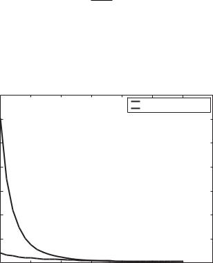
where p is the pressure drop. This means that driving the flow by a pressure gradient is not feasible as depicted on Figure 15.1; note that at a channel height of 10nm three atmospheres of pressure drop are required to drive a flow of Q = 10−6 L/mi n which is a characteristic flow rate in many applications. This is a large pressure drop in a liquid and clearly, a relatively awkward pump would be required to provide this pressure drop.

FIGURE 15.1. Pressure drop and applied voltage as a function of channel height to achieve a flowrate of Q = 10−6 L/mi n in the system of Figure 15.2(b).

The plan of this chapter is as follows. We consider electroosmotic flow for the transport of ionic species; we focus on internal flow since the vast majority of the biomedical applications involve internal flow. In the next section various aspects of electrokinetic phenomena are outlined and then the governing equations are derived; the flow field, the electric field and the mass transfer problems are coupled. We then present results for several different parameters including channel height. The channels considered here are nano-constrained in one dimension. Next we discuss comparisons with experiment and conclude with a discussion of molecular dynamics simulations for probing the limits of continuum theory.

15.2. BACKGROUND

15.2.1. Micro/Nanochannel Systems

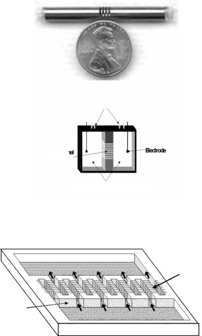
Because it is not feasible to transport fluids in nanochannels using an imposed pressure drop, electroosmosis and electrophoresis are often used. Application areas include rapid bio-molecular analysis; these devices are called lab-on-a-chip. Small drug delivery devices may employ electrokinetic flow to control the rate of flow of drug to the patient. These devices may also be used as biomolecular separators because different ionic species travel at different speeds in these channels. Natural nanochannels exist in cells for the purpose of providing nutrients and discarding waste. In general, these devices act as electroosmotic and/or diffusion pumps (Figure 15.2). The diffusion pump for drug delivery depicted on Figure 15.2 (a) has been tested on rats; the human version is expected to be orders of magnitude smaller. On Figure 15.2 (b) is a sketch of an electroosmotic nanopump whose operation has been documented by iMEDD, Inc. of Columbus, Ohio [8].

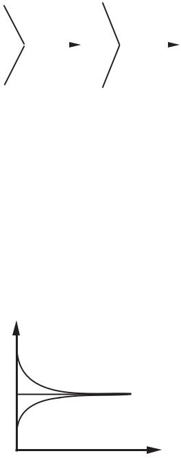
Nanochannel systems applicable to biomolecular analysis require interfacing microchannel arrays with nanochannel arrays. An example is depicted on Figure 15.3. These nanochannels are fabricated by a sacrificial layer lithography method which can produce channels with different surface properties [9]. On Figure 15.3, note that fluid enters from a bath on one side and is forced through several microchannels. The fluid is then forced to turn into a number of much smaller nanochannels which have the ability to sense and interrogate single molecules. Many biomolecules have a characteristic size on the order of 1–5 nm. On the other hand, in the iMEDD device (Figure 15.2(b)), fluid is forced directly into the nanochannels. In most systems of this type, the flow must pass through a micro scale channel into a nanochannel and then into a micro channel again.

One difficulty with modeling these systems is that the voltage drop in the nanochannels is not easily determined. This is because in systems of this type, the electrodes are placed in the baths upstream and downstream of the channels. The electric field must be determined in a complex geometry and in general must be calculated numerically. Moreover, the iMEDD device has over 47,000 nanochannels each of which may operate independently. Clearly each channel cannot be modeled independently in a single numerical simulation.

15.2.2. Previous Work on Electroosmotic Flow

Compared to the amount of work done on flow in micro-channels, there has been relatively little modeling work done on flow in channels whose smallest dimension is on the order

of the electric double layer. In all of this work fully-developed flow is assumed. The problem for channel heights on the order of the electric double layer, that is, for overlapped double layers has been investigated by Verwey [10]. There the solution for the potential is based on a Boltzmann distribution for the number concentration of the ions; the potential is calculated based on a symmetry condition at the centerline. Note that the electric double layer will always be present near charged walls whether or not an external potential is used to drive a bulk motion of the liquid. Qu and Li [11] have recently produced solutions which do not require the Boltzmann distribution, but they also assume symmetry at the centerline; the results show significant differences from the results of Verwey and Overbeek [10]. The results of Qu and Li [11] are valid for low voltages since the Debye-Huckel approximation is invoked.

The first work on the electroosmotic flow problem discussed here appears to have been done by Burgeen and Nakache [12] who also considered the case of overlapped double layers. They produced results for the velocity field and potential for two equally charged ions of valence z; a Boltzmann distribution is assumed for the number of ions in solution. The convective terms in the velocity momentum equation are assumed to be negligible and the solution for the velocity and potential is assumed to be symmetric about the centerline of the channel.

Levine et al. [13] solved the same problem as Burgeen and Nakache [12] and produced results for both thin and overlapping double layers for a single pair of monovalent ions. Again symmetry of the flow with respect to the direction normal to the channel walls is assumed. The current flow is also calculated.

Rice and Whitehead [14] seem to be the first to calculate the electrokinetic flow in a circular tube; they assume a weak electrolyte and so assume the Debye-Huckel approximation holds. Levine et al. [15] also consider flow in a tube under the Debye-Huckel approximation; an analytical solution is found in this case. Stronger electrolyte solutions valid for higher potentials are also condidered using a simplified ad hoc model for the charge density.

Conlisk et al. [16] solve the problem for the ionic mole fractions and the velocity and potential for strong electrolyte solutions and consider the case where there is a potential difference in the direction normal to the channel walls corresponding in some cases to oppositely charged walls. They find that under certain conditions reversed flow may occur in the channel and this situation can significantly reduce the flow rate.

All of the work discussed so far assumes a pair of monovalent ions. However, many biofluids contain a number of other ionic species. As noted above, an example of one of these fluids is the common Phosphate Buffered Saline (PBS) solution. This solution contains five ionic species, with some being divalent. Zheng et al. [17] have solved the entire system of equations numerically; they show that the presence of divalent ions has a significant effect on the flow rate through the channel.

15.2.3. Structure of the Electric Double Layer

Consider the case of an electrolyte mixture which is bounded by a charged wall. If the wall is negatively charged then a surplus of positively charged ions, or cations can be expected to be drawm to the wall. On the other hand, if the wall is positively charged, then it would be expected that there would be a surplus of anions near the wall. The question then becomes, what is the concentration of the cations and anions near a charged surface? This question has vexed chemists for years and the concepts described below are based on qualitative, descriptive models of the region near a charged surface.

FIGURE 15.4. Potential and mole fractions near a negatively charged wall according to the ideas of Helmholtz [18]. Here g denotes the cation mole fraction and f denotes the anion mole fraction.

The electric double layer has been viewed as consisting of a single layer of counterions pinned to the wall outside of which is a layer of mobile coions and counterions. The simplest model for the EDL was originally given by Helmholtz [18] long ago and he assumed that electrical neutrality was achieved in a layer of fixed length. For a negatively charged wall he assumed the distributions of the anions and the cations are linear with distance from the wall as depicted on Figure 15.4.

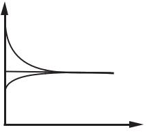
In the Debye-Huckel picture of the electric double layer [19], the influence of the ionic species are equal and opposite so that the wall mole fractions of the coion (anion for a negatively charged wall), f 0 and counterion g0 are symmetric about their asymptotic value far from the wall and the picture is as on Figure 15.5. The Gouy-Chapman [20, 21] model of the electric double layer allows for more counterions to bind to the wall charges so that the counter ions accumulate near the wall. This means that for a negatively charged wall g0 can be much larger than its asymptotic value, whereas f 0, is not much lower than the asymptotic value in the core. This situation is depicted on Figure 15.6. Whether the

g

f

y

FIGURE 15.5. Debye-Huckel [19] picture of the electric double layer. Here g denotes the cation mole fraction and f denotes the anion mole fraction.

g

f

y

FIGURE 15.6. Gouy-Chapman model [20, 21] of the EDL.

Debye-Huckel picture or the Gouy-Chapman model of the EDL obtains depends on the surface charge density with the Debye-Huckel picture occuring at low surface charge densities and the Gouy-Chapman model occuring for higher surface charge densities.

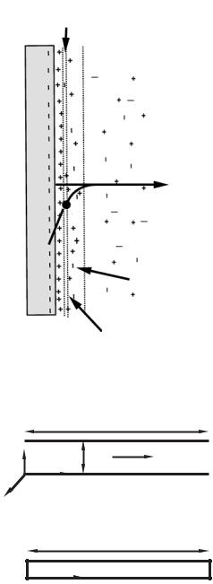
Stern [22] recognized that there are a number of other assumptions embedded in these qualitative and simple models. In the models discussed so far the ions have been assumed to be point charges and the solvent is not modified by the presence of the charges. He proposed that the finite size of the ions affects the value of the potential at the surface. Finite-size ion effects in stagnant solutions are discussed by Bockris and Reddy [6]. Figure 15.7 shows the Stern layer consisting of a single layer of counterions at a negatively charged wall. Stern suggested that the surface potential be evaluated at the surface of shear as shown on Figure 15.7. The potential there is called the ζ potential and is a measured quantity.

15.3. GOVERNING EQUATIONS FOR ELECTROKINETIC FLOW

We consider now the case of flow of an electrolyte mixture in a slit channel for which the width and length of the channel are much bigger than its height as depicted on Figure 15.8. We have in mind the mixture consisting of water and a salt such as sodium chloride, but it is easy to see how to add additional, perhaps multivalent components. We consider the case where the salt is dissociated so that mixture consists of positively and negatively charged ions, say N a+ and Cl−.

In dimensional form, the molar flux of species A for a dilute mixture is a vector and

Here DA B is the diffusion coefficient, c the total concentration, X A is the mole fraction of species A, which can be either the anion or the cation, p is the pressure, MA is the molecular weight, R is the gas constant, T is the temperature, u A is the mobility, z A is the valence, F

the fluid. The mobility u A is defined by u A = RT . The mass transport equation for steady