vk.com/club152685050Submodeling | vk.com/id446425943

a cut through the coarse model. Displacements calculated on the cut boundary of the coarse model are specified as boundary conditions for the submodel.

Submodeling is based on St. Venant's principle, which states that if an actual distribution of forces is replaced by a statically equivalent system, the distribution of stress and strain is altered only near the regions of load application. The principle implies that stress concentration effects are localized around the concentration; therefore, if the boundaries of the submodel are far enough away from the stress concentration, reasonably accurate results can be calculated in the submodel.

The program does not restrict submodeling to structural (stress) analyses only. Submodeling is effective in other disciplines as well. For example, in a magnetic field analysis, you can use submodeling to calculate more accurate magnetic forces in a region of interest.

Aside from the obvious benefit of yielding more accurate results in a region of your model, the submodeling technique has other advantages:

•It reduces, or even eliminates, the need for complicated transition regions in solid finite element models.

•It enables you to experiment with different designs for the region of interest (different fillet radii, for example).

•It helps you in demonstrating the adequacy of mesh refinements.

The following restrictions apply to submodeling:

•It is valid only for solid elements and shell elements.

•The principle behind submodeling assumes that the cut boundaries are far enough away from the stress concentration region. You must verify that this assumption is adequately satisfied.

9.1.1. Nonlinear Submodeling

For load-history-dependent problems (for example, when plastic materials exist), you must cut boundary conditions from the coarse model at multiple substeps to simulate the load history dependency in the fine-mesh model analysis.

In a fine-mesh-model analysis, the cut boundary conditions must be applied as loads at multiple load steps. The more boundary cutting you do, the more accurate are the results of the fine-mesh-model analysis.

Nonlinear submodeling does not apply to shell-to-solid submodels.

9.2. Using Submodeling

The process for using submodeling is as follows:

1.Create and analyze the coarse model.

2.Create the submodel.

3.Perform cut-boundary interpolation.

4.Analyze the submodel.

5. Verify that the distance between the cut boundaries and the stress concentration is adequate.

The steps are explained in detail next.

9.2.1. Create and Analyze the Coarse Model

The first step is to model the entire structure and analyze it.

To easily identify this initial model, it is referred to as the coarse model. This does not mean that the mesh refinement is coarse, only that it is relatively coarse compared to the submodel.

The analysis type may be static (steady-state) or transient and follows the same procedure as described in the individual analysis guides. Some additional points to keep in mind are listed below.

Jobname - Use different job names for the coarse model and the submodel as a precaution against overwriting files, and to easily refer to files from the coarse model during cut-boundary interpolation. To specify a job name, use one of these methods:

Command(s): /FILNAME

GUI: Utility Menu> File> Change Jobname

Element Types -- Only solid and shell elements support the submodeling technique. Your analysis may include other element types (such as beams added as stiffeners), but the cut boundary should only pass through the solids or shells.

A special technique called shell-to-solid submodeling allows you to build your coarse model with shell elements and your submodel with 3-D solid elements. This technique is discussed in Shell-to-Solid Submodels (p. 259).

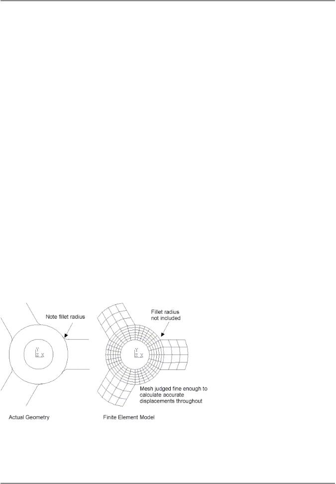
Modeling -- In many cases, the coarse model need not include local details such as fillet radii, as shown in the following figure. However, the finite element mesh must be fine enough to produce a reasonably accurate degree of freedom solution. This is important because the results of the submodel are almost entirely based on interpolated degree of freedom results at the cut boundary.

Figure 9.2: Coarse Model

Initial, coarse model may not need to include many details

Files - Both the results file (Jobname.RST, Jobname.RMG, etc.) and the database file (Jobname.DB, containing the model geometry) are required from the coarse-model analysis. Be sure to save the

vk.com/club152685050Submodeling | vk.com/id446425943

database after solving the coarse model, but before going on to create the submodel. To save the database, use either of these methods:

Command(s): SAVE

GUI: Utility Menu> File> Save as

Utility Menu> File> Save as Jobname.db

9.2.2. Create the Submodel

The submodel is completely independent of the coarse model; therefore, the first step after the initial analysis is to clear the database at the Begin level. To clear the database at the Begin level, use one of these methods:

Command(s): /CLEAR

GUI: Utility Menu> File> Clear & Start New

Also, be sure to use a different job name for the submodel so that the coarse-model files are not overwritten. To specify a job name, use one of these methods:

Command(s): /FILNAME

GUI: Utility Menu> File> Change Jobname

Then enter PREP7 and build the submodel. Some points to remember are:

•Use the same element type (solid or shell) that was used in the coarse model. Also, specify the same element real constants (such as shell thickness) and material properties. (Shell-to-solid submodeling allows you to switch from shell elements in the coarse model to 3-D solid elements in the submodel.)

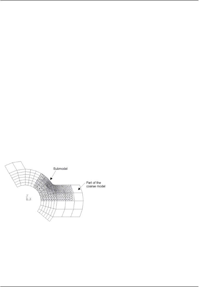
•The location of the submodel (with respect to the global origin) must be the same as the corresponding portion of the coarse model, as shown in Figure 9.3: Submodel Superimposed Over Coarse Mod-

el (p. 248).

Figure 9.3: Submodel Superimposed Over Coarse Model

•Specify appropriate node rotations. Node rotation angles on cut boundary nodes should not be changed after they have been written to the node file in interpolation step 1 (see Perform CutBoundary Interpolation (p. 249)). To specify node rotations, use one of these methods:

Command(s): NROTAT

GUI: Main Menu> Preprocessor> Modeling> Create> Nodes> Rotate Node CS> To Active CS Main Menu> Preprocessor> Modeling> Move/Modify> Rotate Node CS> To Active CS

Be aware that node rotation angles might be changed by application of nodal constraints (DSYM), by transfer of line constraints (SFL), or by transfer of area constraints (SFA), as well as by more obvious methods (NROTAT and NMODIF).

The presence or absence of node rotation angles in the coarse model has no effect upon the submodel.

Loads and boundary conditions for the submodel are covered in subsequent steps.

9.2.3. Perform Cut-Boundary Interpolation

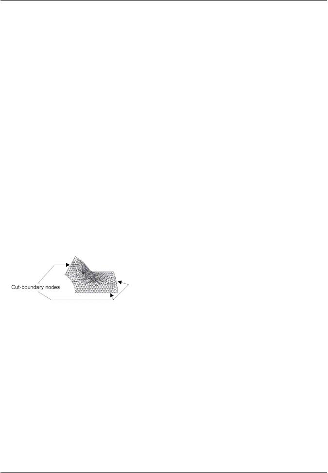
This is the key step in submodeling. You identify the nodes along the cut boundaries, and the program calculates the degree-of-freedom values (displacements, potentials, etc.) at those nodes by interpolating results from the full (coarse) model. For each node of the submodel along the cut boundary, the program uses the appropriate element from the coarse mesh to determine the degree-of-freedom values. These values are then interpolated onto the cut-boundary nodes using the element shape functions.

The following tasks are involved in performing the cut-boundary interpolation:

1.Identify and write the cut-boundary nodes of the submodel to a file (Jobname.NODE by default). You can do this in PREP7 by selecting nodes along the cut boundaries and then using one of these methods to write the nodes to a file:

Command(s): NWRITE

GUI: Main Menu> Preprocessor> Modeling> Create> Nodes> Write Node File

Here is an example of issuing the NWRITE command:

Figure 9.4: Cut Boundaries on the Submodel

At this point, it is worthwhile to discuss temperature interpolation. In an analysis with temperaturedependent material properties, or in a thermal-stress analysis, the temperature distribution

must be the same between the coarse model and the submodel. For such cases, you must also interpolate the temperatures from the coarse model to all nodes in the submodel. To do so, select all submodel nodes and write them to a different file using NWRITE,Filename,Ext. Specify a file name; otherwise, your file of cut-boundary nodes will be overwritten. Step 7 shows the command to do temperature interpolation.

2.Restore the full set of nodes, write the database to Jobname.DB, and leave PREP7. You must write the database to Jobname.DB because you need to continue with the submodel later.

To restore the full set of nodes, use one of these methods:

Command(s): ALLSEL

GUI: Utility Menu> Select> Everything

To write the database to Jobname.DB, use one of these methods:

Command(s): SAVE

GUI: Utility Menu> File> Save as Jobname.db