• Set reasonable limits on the variability for each RV.

Note

The values and hints given below are simply guidelines; none are absolute. Always verify this information with an expert in your organization and adapt it as needed to suit your analysis.

1.4.1.1. Random Input Variables for Monte Carlo Simulations

The number of simulation loops that are required for a Monte Carlo Simulation does not depend on the number of random input variables. The required number of simulation loops only depends on the amount of the scatter of the output parameters and the type of results you expect from the analysis. In a Monte Carlo Simulation, it is a good practice to include all of the random input variables you can think of even if you are not sure about their influence on the random output parameters. Exclude only those random input variables where you are very certain that they have no influence. The probabilistic design system will then automatically tell you which random input variables have turned out to be significant and which one are not. The number of simulations that are necessary in a Monte Carlo analysis to provide that kind of information is usually about 50 to 200. However, the more simulation loops you perform, the more accurate the results will be.

1.4.1.2. Random Input Variables for Response Surface Analyses

The number of simulation loops that are required for a Response Surface analysis depends on the number of random input variables. Therefore, you want to select the most important input variable(s), the ones you know have a significant impact on the random output parameters. If you are unsure which random input variables are important, it is usually a good idea to include all of the random variables you can think of and then perform a Monte Carlo Simulation. After you learn which random input variables are important and therefore should be included in your Response Surface Analysis, you can eliminate those that are unnecessary.

1.4.1.3. Choosing a Distribution for a Random Variable

The type and source of the data you have determines which distribution functions can be used or are best suited to your needs.

1.4.1.3.1. Measured Data

If you have measured data then you first have to know how reliable that data is. Data scatter is not just an inherent physical effect, but also includes inaccuracy in the measurement itself. You must consider that the person taking the measurement might have applied a "tuning" to the data. For example, if the data measured represents a load, the person measuring the load may have rounded the measurement values; this means that the data you receive are not truly the measured values. Depending on the amount of this "tuning," this could provide a deterministic bias in the data that you need to address separately. If possible, you should discuss any bias that might have been built into the data with the person who provided that data to you.

If you are confident about the quality of the data, then how to proceed depends on how much data you have. In a single production field, the amount of data is typically sparse. If you have only few data then it is reasonable to use it only to evaluate a rough figure for the mean value and the standard deviation. In these cases, you could model the random input variable as a Gaussian distribution if the physical effect you model has no lower and upper limit, or use the data and estimate the minimum

vk.com/club152685050Probabi istic Design | vk.com/id446425943

and maximum limit for a uniform distribution. In a mass production field, you probably have a lot of data, in which case you could use a commercial statistical package that will allow you to actually fit a statistical distribution function that best describes the scatter of the data.

1.4.1.3.2. Mean Values, Standard Deviation, Exceedence Values

The mean value and the standard deviation are most commonly used to describe the scatter of data. Frequently, information about a physical quantity is given in the form that its value is; for example, "100±5.5". Often, but not always, this form means that the value "100" is the mean value and "5.5" is the standard deviation. To specify data in this form implies a Gaussian distribution, but you must verify this (a mean value and standard deviation can be provided for any collection of data regardless of the true distribution type). If you have more information (for example, you know that the data must be lognormal distributed), then the PDS allows you to use the mean value and standard deviation for a definition of a lognormal distribution.

Sometimes the scatter of data is also specified by a mean value and an exceedence confidence limit. The yield strength of a material is sometimes given in this way; for example, a 99% exceedence limit based on a 95% confidence level is provided. This means that derived from the measured data we can be sure by 95% that in 99% of all cases the property values will exceed the specified limit and only in 1% of all cases they will drop below the specified limit. The supplier of this information is using mean value, the standard deviation, and the number of samples of the measured data to derive this kind of information. If the scatter of the data is provided in this way, the best way to pursue this further is to

ask for more details from the data supplier. Because the given exceedence limit is based on the measured data and its statistical assessment, the supplier might be able to provide you with the details that were used.

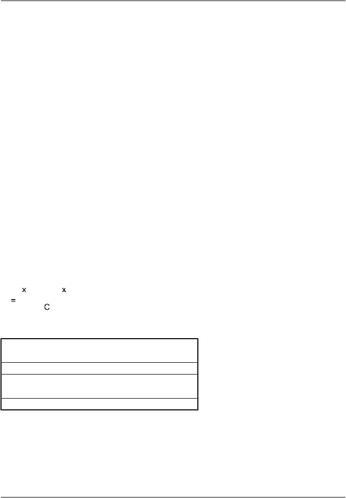
If the data supplier does not give you any further information, then you could consider assuming that the number of measured samples was large. If the given exceedence limit is denoted with x1 - α/2 and the given mean value is denoted with xµ then the standard deviation can be derived from the equation:

where the values for the coefficient C are:

1.4.1.3.3. No Data

In situations where no information is available, there is never just one right answer. Below are hints about which physical quantities are usually described in terms of which distribution functions. This might help you with the particular physical quantity you have in mind. Also below is a list of which distribution functions are usually used for which kind of phenomena. Keep in mind that you might need to choose from multiple options.

Geometric Tolerances

•If you are designing a prototype, you could assume that the actual dimensions of the manufactured parts would be somewhere within the manufacturing tolerances. In this case it is reasonable to use a uniform distribution, where the tolerance bounds provide the lower and upper limits of the distribution function.

•Sometimes the manufacturing process generates a skewed distribution; for example, one half of the tolerance band is more likely to be hit than the other half. This is often the case if missing half of the tolerance band means that rework is necessary, while falling outside the tolerance band on the other

side would lead to the part being scrapped. In this case a Beta distribution is more appropriate.

•Often a Gaussian distribution is used. The fact that the normal distribution has no bounds (it spans minus infinity to infinity), is theoretically a severe violation of the fact that geometrical extensions are described by finite positive numbers only. However, in practice this is irrelevant if the standard deviation is very small compared to the value of the geometric extension, as is typically true for geometric tolerances.

Material Data

•Very often the scatter of material data is described by a Gaussian distribution.

•In some cases the material strength of a part is governed by the "weakest-link-theory". The "weakest- link-theory" assumes that the entire part would fail whenever its weakest spot would fail. for material properties where the "weakest-link" assumptions are valid, then the Weibull distribution might be applicable.

•For some cases, it is acceptable to use the scatter information from a similar material type. Let's assume that you know that a material type very similar to the one you are using has a certain material property with a Gaussian distribution and a standard deviation of ±5% around the measured mean value; then let's assume that for the material type you are using, you only know its mean value. In

this case, you could consider using a Gaussian distribution with a standard deviation of ±5% around the given mean value.

•For temperature-dependent materials it is prudent to describe the randomness by separating the temperature dependency from the scatter effect. In this case you need the mean values of your material property as a function of temperature in the same way that you need this information to perform a deterministic analysis. If M(T) denotes an arbitrary temperature dependent material property then the following approaches are commonly used:

– Multiplication equation:

vk.com/club152685050Probabi istic Design | vk.com/id446425943

Here, (T) denotes the mean value of the material property as a function of temperature. In the "multiplication equation" the mean value function is scaled with a coefficient Crand and this coefficient is a random variable describing the scatter of the material property. In the "additive

equation" a random variable Mrand is added on top of the mean value function (T). The

"linear equation" combines both approaches and here both Crand and Mrand are random variables. However, you should take into account that in general for the "linear equation" approach Crand

and Mrand are, correlated.

Deciding which of these approaches is most suitable to describing the scatter of the temperature dependent material property requires that you have some raw data about this material property. Only by reviewing the raw data and plotting it versus temperature you can tell which approach is the better one.

Load Data

•For loads, you usually only have a nominal or average value. You could ask the person who provided the nominal value the following questions: If we have 1000 components that are operated under real life conditions, what would the lowest load value be that only one of these 1000 components is subjected to and all others have a higher load? What would the most likely load value be, i.e. the value that most of these 1000 components have (or are very close to)? What would the highest load value be that only one of the 1000 components is subjected to and all others have a lower load? To be safe you should ask these questions not only of the person who provided the nominal value, but also to one or more experts who are familiar with how your products are operated under real-life conditions. From all the answers you get, you can then consolidate what the minimum, the most likely, and the maximum value probably is. As verification you can compare this picture with the nominal value that you would use for a deterministic analysis. If the nominal value does not have a conservative bias to it then it should be close to the most likely value. If the nominal value includes a conservative assumption (is biased), then its value is probably close to the maximum value. Finally, you can use a triangular distribution using the minimum, most likely, and maximum values obtained.

•If the load parameter is generated by a computer program then the more accurate procedure is to consider a probabilistic analysis using this computer program as the solver mechanism. Use a probabilistic design technique on that computer program to assess what the scatter of the output parameters are, and apply that data as input to a subsequent analysis. In other words, first run a probabilistic analysis to generate an output range, and then use that output range as input for a subsequent probabilistic analysis.

Here, you have to distinguish if the program that generates the loads is ANSYS itself or your own in-house program. If you have used ANSYS to generate the loads (for example, a thermal

analysis calculating the thermal loads of a structure) then we highly recommend that you include these load calculation steps in the analysis file (and therefore in the probabilistic analysis). In

this case you also need to model the input parameters of these load calculation steps as random input variables. If you have used your own in-house program to generate the loads, you can still integrate the load calculation program in the analysis file (see the /SYS command for details), but you must have an interface between that program and ANSYS that allows the programs to communicate with each other and thus automatically transfer data.

You also have to distinguish if the load values are random fields or single random variables. If the load is different from node to node (element to element) then it is most appropriate to include the program calculating the load in the analysis file. If the load is described by one or very few constant values then

you can also consider performing a probabilistic analysis with the program calculating these load values.