vk.com/club152685050Probabi istic Design | vk.com/id446425943

In our beam example, the maximum deflection and the maximum stress of the beam are random output parameters (RPs). The parameters for these data may be defined as follows:

See the *GET and ETABLE commands for more information.

1.3.1.5. Prepare the Analysis File

If you create your model interactively, you must derive the analysis file from the interactive session. Use the command log or the session log file to do so. For more information about the log files, see Using the ANSYS Session and Command Logs in the Operations Guide.

Note

Do not use the /CLEAR command in your analysis file as this will delete the probabilistic design database during looping. If this happens, the random input variables are no longer recognized during looping and you will get the same (deterministic) results for all simulation loops; however, resume the database using the RESUME command as part of your analysis file. For example, this is helpful if the variations of the random input variables do not require that meshing is done in every loop (because the mesh is not effected). In this case you can mesh your model, save the database, and resume the database at the beginning of the analysis file.

1.3.2. Establish Parameters for Probabilistic Design Analysis

After completing the analysis file, you can begin the probabilistic design analysis. (You may need to reenter the program if you edited the analysis file at the system level.)

When performing probabilistic design interactively, it is advantageous (but optional) to first establish the parameters from the analysis file in the database. (It is unnecessary to do so in batch mode.)

To establish the parameters in the database:

•Resume the database file (Jobname.DB) associated with the analysis file. This establishes your entire model database, including the parameters. To resume the database file:

Command(s): RESUME

GUI: Utility Menu> File> Resume Jobname.db

Utility Menu> File> Resume from

•Read the analysis file to perform the complete analysis. This establishes your entire model database, but might be time-consuming for a large model. To read the analysis file:

Command(s): /INPUT

GUI: Utility Menu> File> Read Input from

•Restore only the parameters from a previously saved parameter file; that is, read in a parameter file that you saved using either the PARSAV command or the Utility Menu> Parameters> Save Parameters menu path. To resume the parameters:

Command(s): PARRES

GUI: Utility Menu> Parameters> Restore Parameters

•Recreate the parameter definitions as they exist in the analysis file. Doing this requires that you know which parameters were defined in the analysis file.

Command(s): *SET

GUI: Utility Menu> Parameters> Scalar Parameters

You may elect to do none of the above, and instead use the PDVAR command to define the parameters that you declare as probabilistic design variables. See Declare Random Input Variables (p. 14) for information on using PDVAR.

Note

The database does not need to contain model information corresponding to the analysis file to perform probabilistic design. The model input is automatically read from the analysis file during probabilistic design looping.

1.3.3. Enter the PDS and Specify the Analysis File

The remaining steps are performed within the PDS processor.

Command(s): /PDS

GUI: Main Menu> Prob Design

In interactive mode, you must specify the analysis file name. This file is used to derive the probabilistic design loop file Jobname.LOOP. The default for the analysis file name is Jobname.pdan. You can also specify a name for the analysis file:

Command(s): PDANL

GUI: Main Menu> Prob Design> Analysis File> Assign

For a probabilistic design run in batch mode, the analysis file is usually the first portion of the batch input stream, from the first line down to the first occurrence of /PDS. In batch mode, the analysis file name defaults to Jobname.BAT (a temporary file containing input copied from the batch input file). Therefore, you normally do not need to specify an analysis filename in batch mode. However, if for some reason you have separated the batch probabilistic design input into two files (one representing

vk.com/club152685050Probabi istic Design | vk.com/id446425943

the analysis and the other containing all probabilistic design operations), then you will need to specify the analysis file using PDANL after entering the PDS (/PDS).

Note

In the analysis file, the /PREP7 and /PDS commands must occur as the first nonblank characters on a line. (Do not use the $ delimiter on a line containing either of these commands.) This requirement is necessary for proper loop file construction.

You cannot assign a different analysis file using the PDANL command after a probabilistic analysis has been performed. This ensures the integrity of the previously generated results with the specified probabilistic model.

The program cannot restrain you from editing the analysis file or exchanging it with system level commands. If you do so, then it is your responsibility to ensure the integrity of the generated results with the definitions in the analysis file. If you are not sure that this integrity is maintained or if you know that it is not, then we recommend that you save the current PDS database via the PDSAVE command and then clear the probabilistic analysis results from the probabilistic design database using the PDCLR, POST command. The PDCLR command does not delete the result files that have been generated; it erases the link to the result files from the database.

In the example of a beam supporting a roof with a snow load you could store the analysis file in a macro named beam.mac. Here, the analysis is specified with the commands:

...

/PDS

PDANL,beam,mac

...

1.3.4. Declare Random Input Variables

The next step is to declare random input variables, that is, specify which parameters are RVs. To declare random input variables:

Command(s): PDVAR

GUI: Main Menu> Prob Design> Prob Definitns> Random Input

If the parameter name that you specify with the PDVAR command is not an existing parameter, the parameter is automatically defined in the database with an initial value of zero.

For random input variables you must specify the type of statistical distribution function used to describe its randomness as well as the parameters of the distribution function. For the distribution type, you can select one of the following:

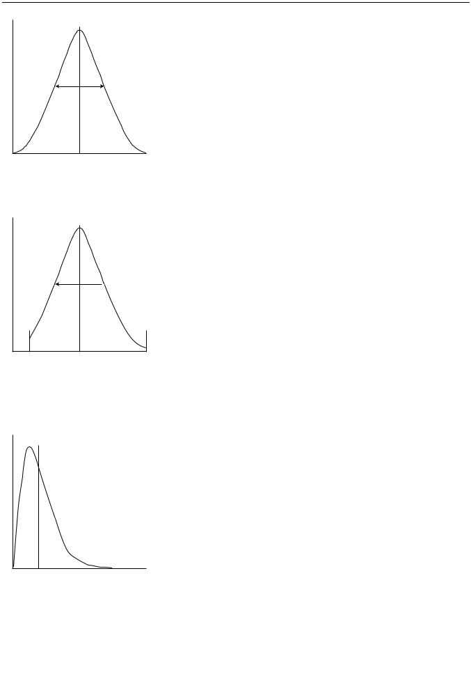
• Gaussian (Normal) (GAUS):

fX(x)

σ

2

µ

x

You provide values for the mean value µ and the standard deviation σ of the random variable x.

• Truncated Gaussian (TGAU):

σ

G

µ

G

You provide the mean value µ and the standard deviation σ of the non-truncated Gaussian distribution and the truncation limits xmin and xmax.

• Lognormal option 1 (LOG1):

µ

You provide values for the mean value µ and the standard deviation σ of the random variable x. The PDS calculates the logarithmic mean ξ and the logarithmic deviation δ:

vk.com/club152685050Probabi istic Design | vk.com/id446425943

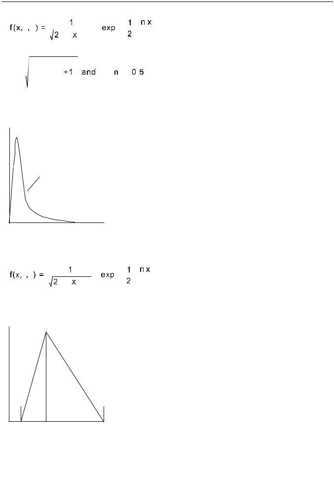
• Lognormal option 2 (LOG2):

fX(x)

ξδ

x

You provide values for the logarithmic mean value ξ and the logarithmic deviation δ. The parameters ξ and δ are the mean value and standard deviation of ln(x):

• Triangular (TRIA):

You provide the minimum value xmin, the most likely value limit xmlv and the maximum value xmax.

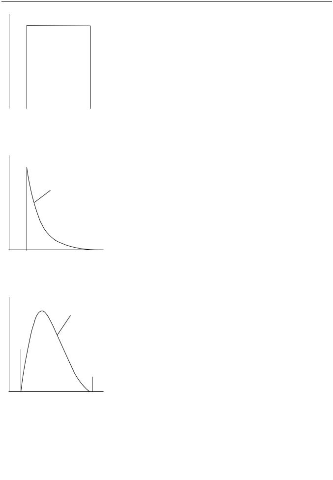
• Uniform (UNIF):

fX(x)

You provide the lower and the upper limit xmin and xmax of the random variable x.

• Exponential (EXPO):

λ

You provide the decay parameter λ and the shift (or lower limit) xmin of the random variable x.

•Beta (BETA):

r,t

You provide the shape parameters r and t and the lower and the upper limit xmin and xmax of the random variable x.

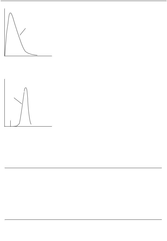
• Gamma (GAMM):

vk.com/club152685050Probabi istic Design | vk.com/id446425943

fX(x)

λ,

k

x

You provide the decay parameter λ and the power parameter k.

• Weibull (Type III smallest) (WEIB):

m, chr

min

You provide the Weibull characteristic value xchr , the Weibull exponent m and the minimum value xmin. Special cases: For xmin = 0 the distribution coincides with a two-parameter Weibull distribution. The Rayleigh distribution is a special case of the Weibull distribution with α = xchr - xmin and m = 2.

You may change the specification of a previously declared random input variable by redefining it. You may also delete a probabilistic design variable (PDVAR,Name,DEL). The delete option does not delete the parameter from the database; it simply deactivates the parameter as a probabilistic design variable.

Note

Changing the probabilistic model by changing a random input variable is not allowed after a probabilistic analysis has been performed. This ensures the integrity of the previously generated results with the specified probabilistic model. If you need to change one or more random input variables (for example, because you learned that some specifications were in-

correct after running an analysis), then we recommend that you save the current PDS database (using the PDSAVE command) and then clear the probabilistic analysis results from the probabilistic design database (using the PDCLR,POST command). The PDCLR command does not delete the result files that have been generated, it simply removes the link to the results file from the database.

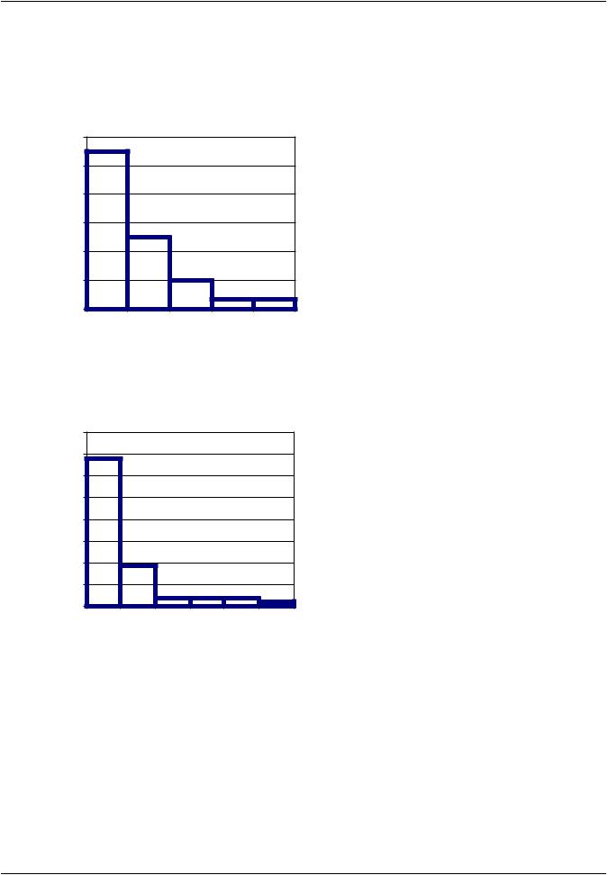
In the example of a beam supporting a roof with a snow load, you could measure the snow height on both ends of the beam 30 different times. Suppose the histograms from these measurements look like the figures given below.

Figure 1.4: Histograms for the Snow Height H1 and H2

From these histograms you can conclude that an exponential distribution is suitable to describe the scatter of the snow height data for H1 and H2. Suppose from the measured data we can evaluate that the average snow height of H1 is 100 mm and the average snow height of H2 is 200 mm. The parameter λ can be directly derived by 1.0 divided by the mean value which leads to λ1 = 1/100 = 0.01 for H1,

and λ1 = 1/200 = 0.005 for H2. From measurements of the Young's modulus you see that the Young's modulus follows a Gaussian distribution with a standard deviation of 5%. Given a mean value of 200,000

N/mm2 for the Young's modulus this gives a standard deviation of 10,000 N/mm2. These definitions can be specified using the following commands: