vk.com/club152685050R tating Structure Analysis | vk.com/id446425943

Example Analysis

For an example of a harmonic analysis for unbalance forces, see Example Unbalance Harmonic Analysis (p. 236).

8.2.3. Orbits

When a structure is rotating about an axis and undergoes vibration motion, the trajectory of a node executed around the axis is generally an ellipse designated as a whirl orbit.

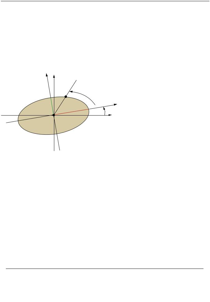
In a local coordinate system xyz where x is the spin axis, the ellipse at node I is defined by semi-major axis A, semi-minor axis B, and phase ψ (PSI), as shown:

Angle ϕ (PHI) defines the initial position of the node (at t = 0). To compare the phases of two nodes of the structure, you can examine the sum ψ + ϕ.

Values YMAX and ZMAX are the maximum displacements along y and z axes, respectively.

You can print out the A, B, PSI, PHI, YMAX, and ZMAX values via a PRORB (print orbits) command. Angles are in degrees and within the range of -180 through +180. The position vector of local axis y in the global coordinate system is printed out along with the elliptical orbit characteristics. You can also animate the orbit (ANHARM) for further examination. For a typical usage example of these commands, see Example Unbalance Harmonic Analysis (p. 236).

To retrieve and store orbits characteristics as parameters, use the *GET command after issuing the PRORB command.

8.3. Using a Rotating Reference Frame

The primary application for a rotating (rather than a stationary) frame of reference is in the field of flexible body dynamics where, generally, the structure has no stationary parts and the entire structure is rotating. Analyses of this type, therefore, consider only the Coriolis force.

Note

The gyroscopic effect is not included in the dynamics equations expressed in a rotating reference frame. Therefore, if the structure contains a part with large inertia - such as a large

disk - the results obtained in the rotating reference frame may not compare well with stationary reference frame results.

ANSYS computes the displacement field with respect to the coordinate system attached to the structure and rotating with it at the specified angular velocity (CORIOLIS,Option = ON,,,RefFrame = OFF).

Elements Supported

The Coriolis matrix and forces are available for the structural elements listed in the notes section of the

CORIOLIS command.

Analysis Types Supported

The following analysis types support rotating structure analysis using a rotating reference frame:

•Static (ANTYPE,STATIC)

Inertia effects are forces computed by multiplying the Coriolis damping matrix by the velocity of the structure.

If you issue the CORIOLIS command in a prestressed analysis, ANSYS does not take the Coriolis force into account in the static portion of the analysis.

–In a large-deflection prestressed analysis (NLGEOM,ON and PSTRES,ON), ANSYS generates the Coriolis matrix and uses it in the subsequent prestressed modal, harmonic, or transient analysis.

–In a small-deflection prestressed analysis (PSTRES,ON only), ANSYS does not generate the Coriolis matrix but still takes the Coriolis force into account in the subsequent prestressed modal, harmonic, or transient analysis.

•Modal (ANTYPE,MODAL)

Support is also available for prestressed modal analysis.

•Transient (ANTYPE,TRANS)

•Harmonic (ANTYPE,HARMIC)

Spin Softening

In a dynamic analysis, the Coriolis matrix and the spin-softening matrix contribute to the gyroscopic moment in the rotating reference frame; therefore, ANSYS includes the spin-softening effect by default

in dynamic analyses whenever you apply the Coriolis effect in the rotating reference frame (CORIOLIS,ON).

Supercritical Spin Softening

As shown by equations (3-77) through (3-79) in the Mechanical APDL Theory Reference, the diagonal coefficients in the stiffness matrix become negative when the rotational velocity is larger than the resonant frequency.

In such cases, the solver may be unable to properly handle the negative definite stiffness matrix. Additional details follow:

vk.com/club152685050R tating Structure Analysis | vk.com/id446425943

•In a static (ANTYPE,STATIC) or a full transient (ANTYPE,TRANS with TRNOPT,FULL), the spin-softening effect is more accurately accounted for by large deflections (NLGEOM,ON). If the stiffness matrix becomes negative definite, ANSYS issues a warning message about the negative pivot.

•In a modal analysis (ANTYPE,MODAL), apply a negative shift (MODOPT,,, FREQB) to extract the possible negative eigenfrequencies.

•If negative frequencies exist, mode-superposition transient and harmonic analyses are not supported .

Coriolis Effect in a Nonlinear Transient Analysis

In a nonlinear transient analysis with large deflection effects (NLGEOM, ON ), rotation motion imparted through either the IC command or the D command contributes the Coriolis effect as part of the nonlinear transient algorithm. The CORIOLIS command should not be activated in this case. However, beam elements (BEAM188 and BEAM189), and pipe elements (PIPE288 and PIPE289 ) may produce approximate results when simulating Coriolis effect as above, due to the approximations involved in their inertia calculations.

Campbell Diagram

Because natural frequencies are subject to sudden changes around critical speeds in a rotating frame, ANSYS, Inc. recommends using a stationary reference frame to create a Campbell diagram (PRCAMP or PLCAMP).

Example Analysis

For examples of a rotating structure analysis using a rotating reference frame, see Example Coriolis Analysis (p. 234), and Example: Piezoelectric Analysis with Coriolis Effect in the Coupled-Field Analysis Guide.

8.4. Choosing the Appropriate Reference Frame Option

The rotating and stationary reference frame approaches have their benefits and limitations. Use this table to choose the best option for your application:

Reference Frame Considerations

Structure must be axisymmetric about the spin axis. Structure need not be axisymmetric about the spin axis.