vk.com/club152685050Probabi istic Design | vk.com/id446425943

1.6.1.4. Print Probabilities

The PDS offers a function where you can determine the cumulative distribution function at any point along the axis of the probabilistic design variable, including an interpolation function so you can evaluate the probabilities between sampling points. This feature is most helpful if you want to evaluate the failure probability or reliability of your component for a very specific and given limit value.

To print probabilities:

Command(s): PDPROB

GUI: Main Menu> Prob Design> Prob Results> Statistics> Probabilities

1.6.1.5. Print Inverse Probabilities

The PDS offers a function where you can probe the cumulative distribution function by specifying a certain probability level; the PDS tells you at which value of the probabilistic design variable this probability will occur. This is helpful if you want to evaluate what limit you should specify to not exceed a certain failure probability, or to specifically achieve a certain reliability for your component.

To print inverse probabilities:

Command(s): PDPINV

GUI: Main Menu> Prob Design> Prob Results> Statistics> Inverse Prob

1.6.2. Trend Postprocessing

Trend postprocessing allows you several options for reviewing your results.

1.6.2.1. Sensitivities

Probabilistic sensitivities are important in allowing you to improve your design toward a more reliable and better quality product, or to save money while maintaining the reliability or quality of your product. You can request a sensitivity plot for any random output parameter in your model.

There is a difference between probabilistic sensitivities and deterministic sensitivities. Deterministic sensitivities are mostly only local gradient information. For example, to evaluate deterministic sensitivities you can vary each input parameters by ±10% (one at a time) while keeping all other input parameters constant, then see how the output parameters react to these variations. As illustrated in the figure below, an output parameter would be considered very sensitive with respect to a certain input parameter if you observe a large change of the output parameter value.

Figure 1.12: Sensitivities

These purely deterministic considerations have various disadvantages that are taken into consideration for probabilistic sensitivities, namely:

•A deterministic variation of an input parameter that is used to determine the gradient usually does not take the physical range of variability into account. An input parameter varied by ±10% is not meaningful for the analysis if ±10% is too much or too little compared with the actual range of physical variability and randomness. In a probabilistic approach the physical range of variability is inherently considered because of the distribution functions for input parameters. Probabilistic sensitivities measure how much the range of scatter of an output parameter is influenced by the scatter of the random input variables. Hence, two effects have an influence on probabilistic sensitivities: the slope of the gradient, plus the width of the scatter range of the random input variables. This is illustrated in the figures below. If a random input variable has a certain given range of scatter, then the scatter of the corresponding random output parameter is larger, and the larger the slope of the

output parameter curve is (first illustration). But remember that an output parameter with a moderate slope can have a significant scatter if the random input variables have a wider range of scatter (second illustration).

Figure 1.13: Range of Scatter

•Gradient information is local information only. It does not take into account that the output parameter may react more or less with respect to variation of input parameters at other locations in the input parameter space. However, the probabilistic approach not only takes the slope at a particular location into account, but also all the values the random output parameter can have within the space of the random input variables.

vk.com/club152685050Probabi istic Design | vk.com/id446425943

•Deterministic sensitivities are typically evaluated using a finite-differencing scheme (varying one parameter at a time while keeping all others fixed). This neglects the effect of interactions between input parameters. An interaction between input parameters exists if the variation of a certain parameter has a greater or lesser effect if at the same time one or more other input parameters change their values as well. In some cases interactions play an important or even dominant role. This is the case if an input parameter is not significant on its own but only in connection with at least one other input parameter. Generally, interactions play an important role in 10% to 15% of typical engineering analysis cases (this figure is problem dependent). If interactions are important, then a deterministic sensitivity analysis can give you completely incorrect results. However, in a probabilistic approach, the results are always based on Monte Carlo simulations, either directly performed using you analysis

model or using response surface equations. Inherently, Monte Carlo simulations always vary all random input variables at the same time; thus if interactions exist then they will always be correctly reflected in the probabilistic sensitivities.

To display sensitivities, the PDS first groups the random input variables into two groups: those having a significant influence on a particular random output parameter and those that are rather insignificant,

based on a statistical significance test. This tests the hypothesis that the sensitivity of a particular random input variable is identical to zero and then calculates the probability that this hypothesis is true. If the probability exceeds a certain significance level (determining that the hypothesis is likely to be true),

then the sensitivity of that random input variable is negligible. The PDS will plot only the sensitivities of the random input variables that are found to be significant. However, insignificant sensitivities are printed in the output window. You can also review the significance probabilities used by the hypothesis test to decide which group a particular random input variable belonged to.

The PDS allows you to visualize sensitivities either as a bar chart, a pie chart, or both. Sensitivities are ranked so the random input variable having the highest sensitivity appears first.

In a bar chart the most important random input variable (with the highest sensitivity) appears in the leftmost position and the others follow to the right in the order of their importance. A bar chart describes the sensitivities in an absolute fashion (taking the signs into account); a positive sensitivity indicates

that increasing the value of the random input variable increases the value of the random output parameter for which the sensitivities are plotted. Likewise, a negative sensitivity indicates that increasing the random input variable value reduces the random output parameter value. In a pie chart, sensitivities are relative to each other.

In a pie chart the most important random input variable (with the highest sensitivity) will appear first after the 12 o'clock position, and the others follow in clockwise direction in the order of their importance.

Using a sensitivity plot, you can answer the following important questions.

How can I make the component more reliable or improve its quality?

If the results for the reliability or failure probability of the component do not reach the expected levels, or if the scatter of an output parameter is too wide and therefore not robust enough for a quality product, then you should make changes to the important input variables first. Modifying an input variable that is insignificant would be waste of time.

Of course you are not in control of all random input parameters. A typical example where you have very limited means of control are material properties. For example, if it turns out that the environmental temperature (outdoor) is the most important input parameter then there is probably nothing you can do. However, even if you find out that the reliability or quality of your product is driven by parameters that you cannot control, this has importance — it is likely that you have a fundamental flaw in your product design! You should watch for influential parameters like these.

If the input variable you want to tackle is a geometry-related parameter or a geometric tolerance, then improving the reliability and quality of your product means that it might be necessary to change to a more accurate manufacturing process or use a more accurate manufacturing machine. If it is a material property, then there is might be nothing you can do about it. However, if you only had a few measurements for a material property and consequently used only a rough guess about its scatter and the material property turns out to be an important driver of product reliability and quality, then it makes sense to collect more raw data. In this way the results of a probabilistic analysis can help you spend your money where it makes the most sense — in areas that affect the reliability and quality of your products the most.

How can I save money without sacrificing the reliability or the quality of the product?

If the results for the reliability or failure probability of the component are acceptable or if the scatter of an output parameter is small and therefore robust enough for a quality product then there is usually the question of how to save money without reducing the reliability or quality. In this case, you should first make changes to the input variables that turned out to be insignificant, because they do not effect

the reliability or quality of your product. If it is the geometrical properties or tolerances that are insignificant, you can consider applying a less expensive manufacturing process. If a material property turns out to be insignificant, then this is not typically a good way to save money, because you are usually not in control of individual material properties. However, the loads or boundary conditions can be a potential for saving money, but in which sense this can be exploited is highly problem dependent.

Command(s): PDSENS

GUI: Main Menu> Prob Design> Prob Results> Trends> Sensitivities

1.6.2.2. Scatter Plots

While the sensitivities point indicate which probabilistic design parameters you need to modify to have an impact on the reliability or failure probability, scatter plots give you a better understanding of how and how far you should modify the input variables. Improving the reliability and quality of a product typically means that the scatter of the relevant random output parameters must be reduced.

The PDS allows you to request a scatter plot of any probabilistic design variable versus any other one,

so you can visualize the relationship between two design variables (input variables or output parameters). This allows you to verify that the sample points really show the pattern of correlation that you specified (if you did so). Typically, random output parameters are correlated as because they are generated by

the same set of random input variables. To support the process of improving the reliability or quality

of your product, a scatter plot showing a random output parameter as a function of the most important random input variable can be very helpful.

When you display a scatter plot, the PDS plots the sampling points and a trendline. For this trendline, the PDS uses a polynomial function and lets you chose the order of the polynomial function. If you plot a random output parameter as a function of a random input variable, then this trendline expresses how much of the scatter on the random output parameter (Y-axis) is controlled by the random input variable (X-axis). The deviations of the sample points from the trendline are caused and controlled by all the other random input variables. If you want to reduce the scatter of the random output parameter to improve reliability and quality, you have two options:

•Reduce the width of the scatter of the most important random input variable(s) (that you have control over).

•Shift the range of the scatter of the most important random input variable(s) (that you have control over).

vk.com/club152685050Probabi istic Design | vk.com/id446425943

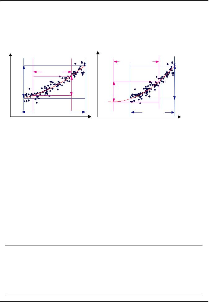
The effect of reducing and shifting the scatter of a random input variable is illustrated in the figures below. "Input range before" denotes the scatter range of the random input variable before the reduction or shifting, and "input range after" illustrates how the scatter range of the random input variable has been modified. In both cases, the trendline tells how much the scatter of the output parameter is affected and in which way if the range of scatter of the random input variable is modified.

Figure 1.14: Effects of Reducing and Shifting Range of Scatter

It depends on your particular problem if either reducing or shifting the range of scatter of a random input variable is preferable. In general, reducing the range of scatter of a random input variable leads to higher costs. A reduction of the scatter range requires a more accurate process in manufacturing or operating the product — the more accurate, the more expensive it is. This might lead you to conclude that shifting the scatter range is a better idea, because it preserves the width of the scatter (which means you can still use the manufacturing or operation process that you have). Below are some considerations if you want to do that:

•Shifting the scatter range of a random input variable can only lead to a reduction of the scatter of a random output parameter if the trendline shows a clear nonlinearity. If the trendline indicates a linear trend (if it is a straight line), then shifting the range of the input variables anywhere along this straight line doesn't make any difference. For this, reducing the scatter range of the random input variable remains your only option.

•It is obvious from the second illustration above that shifting the range of scatter of the random input variable involves an extrapolation beyond the range where you have data. Extrapolation is always difficult and even dangerous if done without care. The more sampling points the trendline is based on the better you can extrapolate. Generally, you should not go more than 30-40% outside of the range of your data. But the advantage of focusing on the important random input variables is that

a slight and careful modification can make a difference.

Note

ANSYS strongly recommends that you redo the entire probabilistic analysis using the new and modified random input variables if you have reduced of shifted the scatter range of any input variables using the procedure and recommendations above. To redo the probabilistic analysis, save the probabilistic model using the PDSAVE command and clear the current probabilistic analysis results using the PDCLR,POST command. Then you can modify the random input variable definitions and redo the probabilistic analysis.