4.7.1.1.3. Hints for Remeshing Multiple Regions

When remeshing using a program-generated new mesh, you can remesh multiple regions at a given substep (referred to as horizontal rezoning) as follows:

1.After starting the remeshing operation (REMESH,START), select a region to remesh.

2.Generate the area for the new mesh (AREMESH).

3.Create the new mesh (AMESH).

4.Select another region (being careful not to overlap regions), generate the area for its new mesh, and create the new mesh on that region.

Repeat the process for as many regions as you wish, but only after issuing the REMESH,START command and before issuing a REMESH,FINISH command (as shown in Understanding the Rezoning Process (p. 92)).

When remeshing two regions or areas that connect to each other, it is best to select them as a single region. If two connected regions must be treated separately, create the mesh for the first region before remeshing the second one.

4.7.1.1.4. Generating a New Mesh

After generating the area (AREMESH) for the selected region, issue the AMESH command to generate the new mesh.

Several preprocessing (/PREP7) commands are available to help you create a good mesh on the selected region. For more information, see Mesh Control (p. 114).

The mesh-control commands are available at any point after issuing a REMESH,START command and before issuing a REMESH,FINISH command.

4.7.1.2. Remeshing Using a Generic New Mesh (2-D and 3-D)

You can remesh using a generic new mesh created by another application. This remeshing method is available for both 2-D and 3-D analyses.

As shown in Figure 4.2: Rezoning Using a Generic New Mesh Generated by Another Application (p. 94), using a generic mesh for the remeshing operation requires the REMESH,READ command, used in place of the commands required for other meshing methods.

To use a new third-party mesh, the mesh file must have a .cdb file format. The .cdb file must have mesh information, but an IGES file (geometry information) is not required. Typically, the new .cdb

mesh is generated from a faceted geometry representation of the boundary of the region to be rezoned.

The element types supported for remeshing with a generic new mesh are given in Rezoning Requirements (p. 90).

The following additional topics related to using a generic new mesh are available:

4.7.1.2.1.Using the REMESH Command with a Generic New Mesh

4.7.1.2.2.Requirements for the Generic New Mesh

4.7.1.2.3.Using the REGE and KEEP Remeshing Options

To study a sample problem, see Example: Rezoning Using a Generic New Mesh (p. 127).

vk.com/club152685050Rezoning | vk.com/id446425943

4.7.1.2.1. Using the REMESH Command with a Generic New Mesh

The commands used for reading in a generic new mesh are shown in Figure 4.2: Rezoning Using a Generic New Mesh Generated by Another Application (p. 94).

Because the REMESH command's READ option reads only generic meshes, all properties of the solid elements in the new mesh are inherited internally from the corresponding underlying solid elements in the old mesh. The program ignores the solid element properties of the new mesh in the .cdb file and calculates them internally depending upon their location in the model; therefore, only the NBLOCK and EBLOCK records of the .cdb file (which define the nodal coordinates and element connectivity, respectively) are read in after issuing a REMESH,READ command.

You can issue multiple REMESH,READ commands for various parts of the mesh in the same rezoning problem (referred to as horizontal rezoning). These multiple regions can be isolated or can touch each other at the boundary, but they cannot overlap. The new mesh, representing multiple regions, can also reside in a single .cdb file.

4.7.1.2.2. Requirements for the Generic New Mesh

The following general requirements must be met by the generic mesh if it is to be a candidate for a new mesh for rezoning:

•The space that the new mesh space occupies, as well as its topology, must conform to that of the old mesh.

•Locations of concentrated forces in the old mesh (usually a node) must be present in the new mesh.

•Limit locations for pressure loads and boundary conditions in the old mesh must be present in the new mesh.

•Limit locations for contact and contact/target element descriptions (in rigid-flex contact and flex-flex contact, respectively) in the old mesh must be present in the new mesh.

The locations of the limits are marked by single nodes in 2-D analyses and by a line of connected nodes in 3-D analyses.

It is not necessary to specify loads, boundary conditions, material properties, etc. on the generic mesh's

.cdb file. The program assigns those values to the new mesh from the model automatically and ignores any specified values. If necessary, you can add new loads later via additional load steps or a restart.

ANSYS, Inc. recommends exporting the deformed old mesh with all discretized boundary information

to a suitable third-party application and, when generating the new mesh, verifying that the node positions of concentrated loads, contact/target region limits, boundary condition and distributed load limits are retained. If these key nodes are not retained, you will be unable to proceed with the analysis.

The new mesh is acceptable even if the smoothed boundary geometry of the new mesh does not correspond exactly to the faceted geometry of the old mesh, as shown in Figure 4.4: Boundary Geometry of a Generic (CDB) New Mesh (p. 103); however, the offset must be very small.

In a 3-D analysis involving contact, the difference of the recovered boundary geometry from the faceted boundary of the old mesh affects mapping results much more so than in a 2-D analysis. Accurate geometry extraction is therefore essential in 3-D rezoning.

Figure 4.4: Boundary Geometry of a Generic (CDB) New Mesh

If the rezoned part has contact/target elements, the program generates those elements automatically for the new mesh, depending on whether the underlying old mesh had the same type of contact/target elements. Isolated rigid target elements in the model remain the same throughout the analysis and cannot be remeshed; however, all contact and target elements associated with solid elements are candidates for remeshing. While it is possible to read in the new contact/target elements of the new mesh from the .cdb file, it is faster and more reliable to read in only the remeshed solid elements and allow the program to generate the new contact/target elements.

The .cdb file of the new mesh must have no line breaks in the NBLOCK and EBLOCK records. Also, while writing the mesh .cdb file, a block file format is necessary (CDWRITE,,,,,,,Fmat, where Fmat = BLOCKED).

4.7.1.2.3. Using the REGE and KEEP Remeshing Options

The REMESH command's REGE option regenerates all node and element numbers on the new mesh using an offset of the highest existing node and element numbers. The KEEP option keeps the similarly numbered nodes and elements in the new and the old meshes unchanged.

Apply Option = KEEP carefully. It assumes that either the new mesh node and element numbers are already offset by the maximum node and element number of the old mesh or that the common node and element numbers in the new mesh and the old mesh match geometrically.

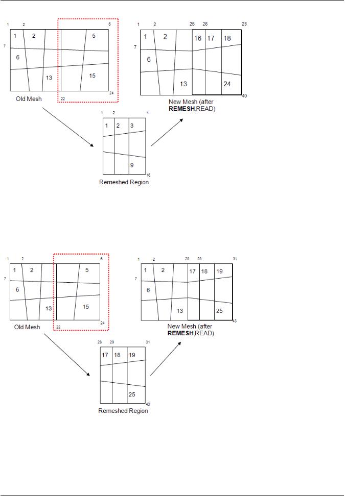
The following figure illustrates how the REMESH command's REGE and KEEP options work:

Figure 4.5: Remeshing Options when Using a Generic (CDB) New Mesh

In this example, a meshed domain with 24 nodes and 15 elements is remeshed using the REMESH command's REGE (default) option. The .cdb file for the new mesh has nodes 1 through 16 and element numbers 1 through 9. After remeshing, these node and element numbers are suitably offset by the maximum node and element numbers (that is, 15 and 24, respectively) of the old mesh.

vk.com/club152685050Rezoning | vk.com/id446425943

The same problem appears in this example. However, the .cdb file for the new mesh has node numbers defined from 28 through 43 and element numbers defined from 17 through 25. In this case, remeshing occurs using the REMESH command's KEEP option, so the node and element numbers are not offset.

For more information, see the REMESH command documentation as it applies to remeshing using a generic mesh created by another application.