vk.com/club152685050Probabi istic Design | vk.com/id446425943

...

PDVAR,H1,EXPO,0.01

PDVAR,H2,EXPO,0.005

PDVAR,YOUNG,GAUS,200000,10000

...

1.3.5. Visualize Random Input Variables

After you define your random input variables, use visual tools to verify them. You can plot individual RVs, and you can obtain specific information about them through an inquiry.

Command(s): PDPLOT, PDINQR

GUI: Main Menu> Prob Design> Prob Definitns> Plot Main Menu> Prob Design> Prob Definitns> Inquire

The PDPLOT command plots the probability density function as well as the cumulative distribution function of a defined random input variable. This allows you to visually check that your definitions are correct.

Use the PDINQR command to inquire about specific information for a defined random input variable by retrieving statistical properties or probing the two function curves that are plotted with the PDPLOT command. For example you can inquire about the mean value of a random input variable or evaluate

at which value the cumulative distribution function reaches a certain probability. The result of this inquiry is stored in a scalar parameter.

1.3.6. Specify Correlations Between Random Variables

In a probabilistic design analysis, random input variables can have specific relationships to each other, called correlations. If two (or more) random input variables are statistically dependent on each other, then there is a correlation between those variables.

To define these correlations:

Command(s): PDCORR

GUI: Main Menu> Prob Design> Prob Definitns> Correlation

You specify the two random input variables for which you want to specify a correlation, and the correlation coefficient (between -1 and 1). To remove a correlation, enter DEL in the correlation coefficient field (PDCORR,Name1,Name2,DEL)

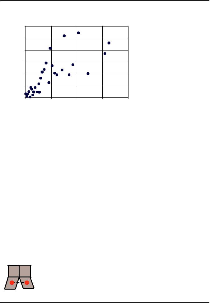
In the example of a beam supporting a roof with a snow load, the data for the snow height indicates that there is a correlation between the snow height at one end versus the snow height at the other end. This is due to the fact that it is unlikely that one end of the beam has very little snow (or no snow at all) at the same time that the other end carries a huge amount of snow. In the average the two snow heights tend to be similar. This correlation is obvious if you plot the measured data values for H2 versus the data value for H1. This scatter plot looks like this:

Figure 1.5: A Scatter Plot of Snow Height H1 vs. H2

Performing a statistical evaluation of the data, we can conclude that the linear correlation coefficient between the values of H1 and H2 is about 0.8. You can define this correlation using the commands:

...

PDVAR,H1,EXPO,0.01

PDVAR,H2,EXPO,0.005

PDCORR,H1,H2,0.8

...

You may have a more complex correlation where you have a spatial dependency. If so, you can use the PDCFLD command to calculate a correlation field and store it into an array.

Random fields are random effects with a spatial distribution; the value of a random field not only varies from simulation to simulation at any given location, but also from location to location. The correlation field describes the correlation coefficient between two different spatial locations. Random fields can be either based on element properties (typically material) or nodal properties (typically surface shape defined by nodal coordinates). Hence, random fields are either associated with the selected nodes or the selected elements. If a random field is associated with elements, then the correlation coefficients

of the random field are calculated based on the distance of the element centroids.

Note that for correlation fields, the “domain distance” D({xi} , {xj}) is not the spatial distance |{xi} - {xj}|, but the length of a path between {xi} and {xj} that always remains inside the finite element domain. However, exceptions are possible in extreme meshing cases. For elements that share at least one node, the PDCFLD evaluates the distance by directly connecting the element centroids with a straight line.

If these neighboring elements form a sharp inward corner then it is possible that the “domain distance” path lies partly outside the finite element domain, as illustrated below.

vk.com/club152685050Probabi istic Design | vk.com/id446425943

After the correlation coefficients have been calculated and stored in a parameter (PDCFLD,ParR), then you can use the PDCORR command to define the correlations between the elements of the random field.

Note

When specifying one variable (A) with correlations to two or more other variables (B, C, etc.), be certain that you consider the relationship implied between the other variables B and C, etc. If you specify high correlations between A and B and A and C, without specifying the relationship between B and C, you might receive an error. Specifying a relatively high correlation between A and B, with only a moderate correlation between A and C might work because the logical correlation between B and C could still be low or nonexistent.

Example

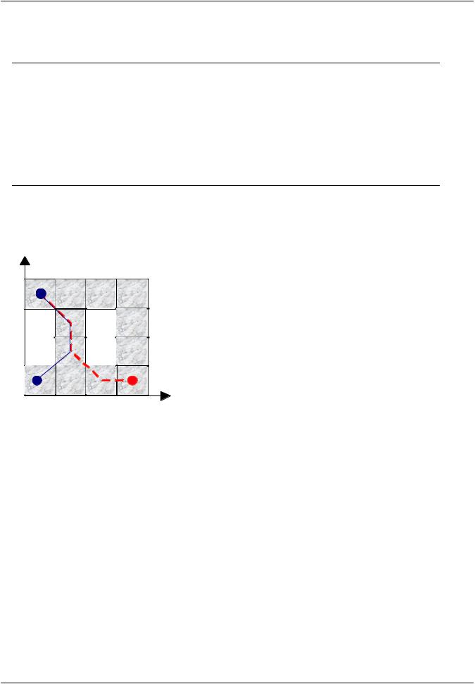
The structure illustrated below is modeled with 12 elements. We will evaluate the domain distances of the element centroids.

First, build the finite element structure:

...

/PREP7

et,1,shell181,,,2 ! create the nodes N,1,0,4

N,2,1,4

N,3,2,4

N,4,3,4

N,5,4,4

N,6,0,3

N,7,1,3

N,8,2,3

N,9,3,3

N,10,4,3

N,11,1,2

N,12,2,2

N,13,3,2

N,14,4,2

N,15,0,1

N,16,1,1

N,17,2,1

N,18,3,1

N,19,4,1

N,20,0,0

N,21,1,0

N,22,2,0

N,23,3,0

N,24,4,0

! create the elements E,1,2,7,6

E,2,3,8,7

E,3,4,9,8

E,4,5,10,9

E,7,8,12,11

E,9,10,14,13

E,11,12,17,16

E,13,14,19,18

E,15,16,21,20

E,16,17,22,21

E,17,18,23,22

E,18,19,24,23

...

Next, calculate the domain distances and store the results in the array “elemdist”:

...

/PDS

PDCFLD,elemdist,ELEM,DIST

...

Finally, get all the element domain distances and print them:

...

*GET,numsel,ELEM,0,COUNT ! Get the number of selected elements

!

!Outer loop through all selected elements from first to last index=0

elem1=0

!Pipe output to file

The print out will show that for the structure illustrated above the "domain distance" between the element centroids of elements 1 and 9 is 3.8284 and between the element centroids of elements 1 and 12 it is 4.8284. The paths related to these distances are sketched in the illustration with a solid line and a dashed line respectively. In this example there are 12 elements, thus the array "elemdist" has a length of 12*(12- 1)/2 = 66.

1.3.7. Specify Random Output Parameters

After declaring your input variables and correlations among them you must define the random output parameters. The random output parameters (RPs) are results parameters that you are interested in. To define random output parameters:

Command(s): PDVAR,Name,RESP