

- •Table of Contents
- •Chapter 1: Probabilistic Design
- •1.1. Understanding Probabilistic Design
- •1.1.1. Traditional (Deterministic) vs. Probabilistic Design Analysis Methods
- •1.1.2. Reliability and Quality Issues
- •1.2. Probabilistic Design Terminology
- •1.3. Using Probabilistic Design
- •1.3.1. Create the Analysis File
- •1.3.1.1. Example Problem Description
- •1.3.1.2. Build the Model Parametrically
- •1.3.1.3. Obtain the Solution
- •1.3.1.4. Retrieve Results and Assign as Output Parameters
- •1.3.1.5. Prepare the Analysis File
- •1.3.2. Establish Parameters for Probabilistic Design Analysis
- •1.3.3. Enter the PDS and Specify the Analysis File
- •1.3.4. Declare Random Input Variables
- •1.3.5. Visualize Random Input Variables
- •1.3.6. Specify Correlations Between Random Variables
- •1.3.7. Specify Random Output Parameters
- •1.3.8. Select a Probabilistic Design Method
- •1.3.8.1. Probabilistic Method Determination Wizard
- •1.3.9. Execute Probabilistic Analysis Simulation Loops
- •1.3.9.1. Probabilistic Design Looping
- •1.3.9.2. Serial Analysis Runs
- •1.3.9.3. PDS Parallel Analysis Runs
- •1.3.9.3.1. Machine Configurations
- •1.3.9.3.1.1. Choosing Slave Machines
- •1.3.9.3.1.2. Using the Remote Shell Option
- •1.3.9.3.1.3. Using the Connection Port Option
- •1.3.9.3.1.4. Configuring the Master Machine
- •1.3.9.3.1.5. Host setup using port option
- •1.3.9.3.1.6. Host and Product selection for a particular analysis
- •1.3.9.3.2. Files Needed for Parallel Run
- •1.3.9.3.3. Controlling Server Processes
- •1.3.9.3.4. Initiate Parallel Run
- •1.3.10. Fit and Use Response Surfaces
- •1.3.10.1. About Response Surface Sets
- •1.3.10.2. Fitting a Response Surface
- •1.3.10.3. Plotting a Response Surface
- •1.3.10.4. Printing a Response Surface
- •1.3.10.5. Generating Monte Carlo Simulation Samples on the Response Surfaces
- •1.3.11. Review Results Data
- •1.3.11.1. Viewing Statistics
- •1.3.11.2. Viewing Trends
- •1.3.11.3. Creating Reports
- •1.4. Guidelines for Selecting Probabilistic Design Variables
- •1.4.1. Choosing and Defining Random Input Variables
- •1.4.1.1. Random Input Variables for Monte Carlo Simulations
- •1.4.1.2. Random Input Variables for Response Surface Analyses
- •1.4.1.3. Choosing a Distribution for a Random Variable
- •1.4.1.3.1. Measured Data
- •1.4.1.3.2. Mean Values, Standard Deviation, Exceedence Values
- •1.4.1.3.3. No Data
- •1.4.1.4. Distribution Functions
- •1.4.2. Choosing Random Output Parameters
- •1.5. Probabilistic Design Techniques
- •1.5.1. Monte Carlo Simulations
- •1.5.1.1. Direct Sampling
- •1.5.1.2. Latin Hypercube Sampling
- •1.5.1.3. User-Defined Sampling
- •1.5.2. Response Surface Analysis Methods
- •1.5.2.1. Central Composite Design Sampling
- •1.5.2.2. Box-Behnken Matrix Sampling
- •1.5.2.3. User-Defined Sampling
- •1.6. Postprocessing Probabilistic Analysis Results
- •1.6.1. Statistical Postprocessing
- •1.6.1.1. Sample History
- •1.6.1.2. Histogram
- •1.6.1.3. Cumulative Distribution Function
- •1.6.1.4. Print Probabilities
- •1.6.1.5. Print Inverse Probabilities
- •1.6.2. Trend Postprocessing
- •1.6.2.1. Sensitivities
- •1.6.2.2. Scatter Plots
- •1.6.2.3. Correlation Matrix
- •1.6.3. Generating an HTML Report
- •1.7. Multiple Probabilistic Design Executions
- •1.7.1. Saving the Probabilistic Design Database
- •1.7.2. Restarting a Probabilistic Design Analysis
- •1.7.3. Clearing the Probabilistic Design Database
- •1.8. Example Probabilistic Design Analysis
- •1.8.1. Problem Description
- •1.8.2. Problem Specifications
- •1.8.2.1. Problem Sketch
- •1.8.3. Using a Batch File for the Analysis
- •1.8.4. Using the GUI for the PDS Analysis
- •Chapter 2: Variational Technology
- •2.1. Harmonic Sweep Using VT Accelerator
- •2.1.1. Structural Elements Supporting Frequency-Dependent Properties
- •2.1.2. Harmonic Sweep for Structural Analysis with Frequency-Dependent Material Properties
- •2.1.2.1. Beam Example
- •Chapter 3: Adaptive Meshing
- •3.1. Prerequisites for Adaptive Meshing
- •3.2. Employing Adaptive Meshing
- •3.3. Modifying the Adaptive Meshing Process
- •3.3.1. Selective Adaptivity
- •3.3.2. Customizing the ADAPT Macro with User Subroutines
- •3.3.2.1. Creating a Custom Meshing Subroutine (ADAPTMSH.MAC)
- •3.3.2.2. Creating a Custom Subroutine for Boundary Conditions (ADAPTBC.MAC)
- •3.3.2.3. Creating a Custom Solution Subroutine (ADAPTSOL.MAC)
- •3.3.2.4. Some Further Comments on Custom Subroutines
- •3.3.3. Customizing the ADAPT Macro (UADAPT.MAC)
- •3.4. Adaptive Meshing Hints and Comments
- •3.5. Where to Find Examples
- •Chapter 4: Rezoning
- •4.1. Benefits and Limitations of Rezoning
- •4.1.1. Rezoning Limitations
- •4.2. Rezoning Requirements
- •4.3. Understanding the Rezoning Process
- •4.3.1. Overview of the Rezoning Process Flow
- •4.3.2. Key Commands Used in Rezoning
- •4.4. Step 1: Determine the Substep to Initiate Rezoning
- •4.5. Step 2. Initiate Rezoning
- •4.6. Step 3: Select a Region to Remesh
- •4.7. Step 4: Perform the Remeshing Operation
- •4.7.1. Choosing a Remeshing Method
- •4.7.1.1. Remeshing Using a Program-Generated New Mesh (2-D)
- •4.7.1.1.1. Creating an Area to Remesh
- •4.7.1.1.2. Using Nodes From the Old Mesh
- •4.7.1.1.3. Hints for Remeshing Multiple Regions
- •4.7.1.1.4. Generating a New Mesh
- •4.7.1.2. Remeshing Using a Generic New Mesh (2-D and 3-D)
- •4.7.1.2.1. Using the REMESH Command with a Generic New Mesh
- •4.7.1.2.2. Requirements for the Generic New Mesh
- •4.7.1.2.3. Using the REGE and KEEP Remeshing Options
- •4.7.1.3. Remeshing Using Manual Mesh Splitting (2-D and 3-D)
- •4.7.1.3.1. Understanding Mesh Splitting
- •4.7.1.3.2. Geometry Details for Mesh Splitting
- •4.7.1.3.3. Using the REMESH Command for Mesh Splitting
- •4.7.1.3.4. Mesh-Transition Options for 2-D Mesh Splitting
- •4.7.1.3.5. Mesh-Transition Options for 3-D Mesh Splitting
- •4.7.1.3.7. Improving Tetrahedral Element Quality via Mesh Morphing
- •4.7.2. Mesh Control
- •4.7.3. Remeshing Multiple Regions at the Same Substep
- •4.8. Step 5: Verify Applied Contact Boundaries, Surface-Effect Elements, Loads, and Boundary Conditions
- •4.8.1. Contact Boundaries
- •4.8.2. Surface-Effect Elements
- •4.8.3. Pressure and Contiguous Displacements
- •4.8.4. Forces and Isolated Applied Displacements
- •4.8.5. Nodal Temperatures
- •4.8.6. Other Boundary Conditions and Loads
- •4.9. Step 6: Automatically Map Variables and Balance Residuals
- •4.9.1. Mapping Solution Variables
- •4.9.2. Balancing Residual Forces
- •4.9.3. Interpreting Mapped Results
- •4.9.4. Handling Convergence Difficulties
- •4.10. Step 7: Perform a Multiframe Restart
- •4.11. Repeating the Rezoning Process if Necessary
- •4.11.1. File Structures for Repeated Rezonings
- •4.12. Postprocessing Rezoning Results
- •4.12.1. The Database Postprocessor
- •4.12.1.1. Listing the Rezoning Results File Summary
- •4.12.1.2. Animating the Rezoning Results
- •4.12.1.3. Using the Results Viewer for Rezoning
- •4.12.2. The Time-History Postprocessor
- •4.13. Rezoning Restrictions
- •4.14. Rezoning Examples
- •4.14.1. Example: Rezoning Using a Program-Generated New Mesh
- •4.14.1.1. Initial Input for the Analysis
- •4.14.1.2. Rezoning Input for the Analysis
- •4.14.2. Example: Rezoning Using a Generic New Mesh
- •4.14.2.1. Initial Input for the Analysis
- •4.14.2.2. Exporting the Distorted Mesh as a CDB File
- •4.14.2.3. Importing the File into ANSYS ICEM CFD and Generating a New Mesh
- •4.14.2.4. Rezoning Using the New CDB Mesh
- •Chapter 5: Mesh Nonlinear Adaptivity
- •5.1. Mesh Nonlinear Adaptivity Benefits, Limitations and Requirements
- •5.1.1. Rubber Seal Simulation
- •5.1.2. Crack Simulation
- •5.2. Understanding the Mesh Nonlinear Adaptivity Process
- •5.2.1. Checking Nonlinear Adaptivity Criteria
- •5.2.1.1. Defining Element Components
- •5.2.1.2. Defining Nonlinear Adaptivity Criteria
- •5.2.1.3. Defining Criteria-Checking Frequency
- •5.3. Mesh Nonlinear Adaptivity Criteria
- •5.3.1. Energy-Based
- •5.3.2. Position-Based
- •5.3.3. Contact-Based
- •5.3.4. Frequency of Criteria Checking
- •5.4. How a New Mesh Is Generated
- •5.5. Convergence at Substeps with the New Mesh
- •5.6. Controlling Mesh Nonlinear Adaptivity
- •5.7. Postprocessing Mesh Nonlinear Adaptivity Results
- •5.8. Mesh Nonlinear Adaptivity Examples
- •5.8.1. Example: Rubber Seal Simulation
- •5.8.2. Example: Crack Simulation
- •Chapter 6: 2-D to 3-D Analysis
- •6.1. Benefits of 2-D to 3-D Analysis
- •6.2. Requirements for a 2-D to 3-D Analysis
- •6.3. Overview of the 2-D to 3-D Analysis Process
- •6.3.1. Overview of the 2-D to 3-D Analysis Process Flow
- •6.3.2. Key Commands Used in 2-D to 3-D Analysis
- •6.4. Performing a 2-D to 3-D Analysis
- •6.4.1. Step 1: Determine the Substep to Initiate
- •6.4.2. Step 2: Initiate the 2-D to 3-D Analysis
- •6.4.3. Step 3: Extrude the 2-D Mesh to the New 3-D Mesh
- •6.4.4. Step 4: Map Solution Variables from 2-D to 3-D Mesh
- •6.4.5. Step 5: Perform an Initial-State-Based 3-D Analysis
- •6.5. 2-D to 3-D Analysis Restrictions
- •Chapter 7: Cyclic Symmetry Analysis
- •7.1. Understanding Cyclic Symmetry Analysis
- •7.1.1. How the Program Automates a Cyclic Symmetry Analysis
- •7.1.2. Commands Used in a Cyclic Symmetry Analysis
- •7.2. Cyclic Modeling
- •7.2.1. The Basic Sector
- •7.2.2. Edge Component Pairs
- •7.2.2.1. CYCOPT Auto Detection Tolerance Adjustments for Difficult Cases
- •7.2.2.2. Identical vs. Dissimilar Edge Node Patterns
- •7.2.2.3. Unmatched Nodes on Edge-Component Pairs
- •7.2.2.4. Identifying Matching Node Pairs
- •7.2.3. Modeling Limitations
- •7.2.4. Model Verification (Preprocessing)
- •7.3. Solving a Cyclic Symmetry Analysis
- •7.3.1. Understanding the Solution Architecture
- •7.3.1.1. The Duplicate Sector
- •7.3.1.2. Coupling and Constraint Equations (CEs)
- •7.3.1.3. Non-Cyclically Symmetric Loading
- •7.3.1.3.1. Specifying Non-Cyclic Loading
- •7.3.1.3.2. Commands Affected by Non-Cyclic Loading
- •7.3.1.3.3. Plotting and Listing Non-Cyclic Boundary Conditions
- •7.3.1.3.4. Graphically Picking Non-Cyclic Boundary Conditions
- •7.3.2. Solving a Static Cyclic Symmetry Analysis
- •7.3.3. Solving a Modal Cyclic Symmetry Analysis
- •7.3.3.1. Understanding Harmonic Index and Nodal Diameter
- •7.3.3.2. Solving a Stress-Free Modal Analysis
- •7.3.3.3. Solving a Prestressed Modal Analysis
- •7.3.3.4. Solving a Large-Deflection Prestressed Modal Analysis
- •7.3.3.4.1. Solving a Large-Deflection Prestressed Modal Analysis with VT Accelerator
- •7.3.4. Solving a Linear Buckling Cyclic Symmetry Analysis
- •7.3.5. Solving a Harmonic Cyclic Symmetry Analysis
- •7.3.5.1. Solving a Full Harmonic Cyclic Symmetry Analysis
- •7.3.5.1.1. Solving a Prestressed Full Harmonic Cyclic Symmetry Analysis
- •7.3.5.2. Solving a Mode-Superposition Harmonic Cyclic Symmetry Analysis
- •7.3.5.2.1. Perform a Static Cyclic Symmetry Analysis to Obtain the Prestressed State
- •7.3.5.2.2. Perform a Linear Perturbation Modal Cyclic Symmetry Analysis
- •7.3.5.2.3. Restart the Modal Analysis to Create the Desired Load Vector from Element Loads
- •7.3.5.2.4. Obtain the Mode-Superposition Harmonic Cyclic Symmetry Solution
- •7.3.5.2.5. Review the Results
- •7.3.6. Solving a Magnetic Cyclic Symmetry Analysis
- •7.3.7. Database Considerations After Obtaining the Solution
- •7.3.8. Model Verification (Solution)
- •7.4. Postprocessing a Cyclic Symmetry Analysis
- •7.4.1. General Considerations
- •7.4.1.1. Using the /CYCEXPAND Command
- •7.4.1.1.1. /CYCEXPAND Limitations
- •7.4.1.2. Result Coordinate System
- •7.4.2. Modal Solution
- •7.4.2.1. Real and Imaginary Solution Components
- •7.4.2.2. Expanding the Cyclic Symmetry Solution
- •7.4.2.3. Applying a Traveling Wave Animation to the Cyclic Model
- •7.4.2.4. Phase Sweep of Repeated Eigenvector Shapes
- •7.4.3. Static, Buckling, and Full Harmonic Solutions
- •7.4.4. Mode-Superposition Harmonic Solution
- •7.5. Example Modal Cyclic Symmetry Analysis
- •7.5.1. Problem Description
- •7.5.2. Problem Specifications
- •7.5.3. Input File for the Analysis
- •7.5.4. Analysis Steps
- •7.6. Example Buckling Cyclic Symmetry Analysis
- •7.6.1. Problem Description
- •7.6.2. Problem Specifications
- •7.6.3. Input File for the Analysis
- •7.6.4. Analysis Steps
- •7.6.5. Solve For Critical Strut Temperature at Load Factor = 1.0
- •7.7. Example Harmonic Cyclic Symmetry Analysis
- •7.7.1. Problem Description
- •7.7.2. Problem Specifications
- •7.7.3. Input File for the Analysis
- •7.7.4. Analysis Steps
- •7.8. Example Magnetic Cyclic Symmetry Analysis
- •7.8.1. Problem Description
- •7.8.2. Problem Specifications
- •7.8.3. Input file for the Analysis
- •Chapter 8: Rotating Structure Analysis
- •8.1. Understanding Rotating Structure Dynamics
- •8.2. Using a Stationary Reference Frame
- •8.2.1. Campbell Diagram
- •8.2.2. Harmonic Analysis for Unbalance or General Rotating Asynchronous Forces
- •8.2.3. Orbits
- •8.3. Using a Rotating Reference Frame
- •8.4. Choosing the Appropriate Reference Frame Option
- •8.5. Example Campbell Diagram Analysis
- •8.5.1. Problem Description
- •8.5.2. Problem Specifications
- •8.5.3. Input for the Analysis
- •8.5.4. Analysis Steps
- •8.6. Example Coriolis Analysis
- •8.6.1. Problem Description
- •8.6.2. Problem Specifications
- •8.6.3. Input for the Analysis
- •8.6.4. Analysis Steps
- •8.7. Example Unbalance Harmonic Analysis
- •8.7.1. Problem Description
- •8.7.2. Problem Specifications
- •8.7.3. Input for the Analysis
- •8.7.4. Analysis Steps
- •Chapter 9: Submodeling
- •9.1. Understanding Submodeling
- •9.1.1. Nonlinear Submodeling
- •9.2. Using Submodeling
- •9.2.1. Create and Analyze the Coarse Model
- •9.2.2. Create the Submodel
- •9.2.3. Perform Cut-Boundary Interpolation
- •9.2.4. Analyze the Submodel
- •9.3. Example Submodeling Analysis Input
- •9.3.1. Submodeling Analysis Input: No Load-History Dependency
- •9.3.2. Submodeling Analysis Input: Load-History Dependency
- •9.4. Shell-to-Solid Submodels
- •9.5. Where to Find Examples
- •Chapter 10: Substructuring
- •10.1. Benefits of Substructuring
- •10.2. Using Substructuring
- •10.2.1. Step 1: Generation Pass (Creating the Superelement)
- •10.2.1.1. Building the Model
- •10.2.1.2. Applying Loads and Creating the Superelement Matrices
- •10.2.1.2.1. Applicable Loads in a Substructure Analysis
- •10.2.2. Step 2: Use Pass (Using the Superelement)
- •10.2.2.1. Clear the Database and Specify a New Jobname
- •10.2.2.2. Build the Model
- •10.2.2.3. Apply Loads and Obtain the Solution
- •10.2.3. Step 3: Expansion Pass (Expanding Results Within the Superelement)
- •10.3. Sample Analysis Input
- •10.4. Top-Down Substructuring
- •10.5. Automatically Generating Superelements
- •10.6. Nested Superelements
- •10.7. Prestressed Substructures
- •10.7.1. Static Analysis Prestress
- •10.7.2. Substructuring Analysis Prestress
- •10.8. Where to Find Examples
- •Chapter 11: Component Mode Synthesis
- •11.1. Understanding Component Mode Synthesis
- •11.1.1. CMS Methods Supported
- •11.1.2. Solvers Used in Component Mode Synthesis
- •11.2. Using Component Mode Synthesis
- •11.2.1. The CMS Generation Pass: Creating the Superelement
- •11.2.2. The CMS Use and Expansion Passes
- •11.2.3. Superelement Expansion in Transformed Locations
- •11.2.4. Plotting or Printing Mode Shapes
- •11.3. Example Component Mode Synthesis Analysis
- •11.3.1. Problem Description
- •11.3.2. Problem Specifications
- •11.3.3. Input for the Analysis: Fixed-Interface Method
- •11.3.4. Analysis Steps: Fixed-Interface Method
- •11.3.5. Input for the Analysis: Free-Interface Method
- •11.3.6. Analysis Steps: Free-Interface Method
- •11.3.7. Input for the Analysis: Residual-Flexible Free-Interface Method
- •11.3.8. Analysis Steps: Residual-Flexible Free-Interface Method
- •11.3.9. Example: Superelement Expansion in a Transformed Location
- •11.3.9.1. Analysis Steps: Superelement Expansion in a Transformed Location
- •11.3.10. Example: Reduce the Damping Matrix and Compare Full and CMS Results with RSTMAC
- •Chapter 12: Rigid-Body Dynamics and the ANSYS-ADAMS Interface
- •12.1. Understanding the ANSYS-ADAMS Interface
- •12.2. Building the Model
- •12.3. Modeling Interface Points
- •12.4. Exporting to ADAMS
- •12.4.1. Exporting to ADAMS via Batch Mode
- •12.4.2. Verifying the Results
- •12.5. Running the ADAMS Simulation
- •12.6. Transferring Loads from ADAMS
- •12.6.1. Transferring Loads on a Rigid Body
- •12.6.1.1. Exporting Loads in ADAMS
- •12.6.1.2. Importing Loads
- •12.6.1.3. Importing Loads via Commands
- •12.6.1.4. Reviewing the Results
- •12.6.2. Transferring the Loads of a Flexible Body
- •12.7. Methodology Behind the ANSYS-ADAMS Interface
- •12.7.1. The Modal Neutral File
- •12.7.2. Adding Weak Springs
- •12.8. Example Rigid-Body Dynamic Analysis
- •12.8.1. Problem Description
- •12.8.2. Problem Specifications
- •12.8.3. Command Input
- •Chapter 13: Element Birth and Death
- •13.1. Elements Supporting Birth and Death
- •13.2. Understanding Element Birth and Death
- •13.3. Element Birth and Death Usage Hints
- •13.3.1. Changing Material Properties
- •13.4. Using Birth and Death
- •13.4.1. Build the Model
- •13.4.2. Apply Loads and Obtain the Solution
- •13.4.2.1. Define the First Load Step
- •13.4.2.1.1. Sample Input for First Load Step
- •13.4.2.2. Define Subsequent Load Steps
- •13.4.2.2.1. Sample Input for Subsequent Load Steps
- •13.4.3. Review the Results
- •13.4.4. Use Analysis Results to Control Birth and Death
- •13.4.4.1. Sample Input for Deactivating Elements
- •13.5. Where to Find Examples
- •Chapter 14: User-Programmable Features and Nonstandard Uses
- •14.1. User-Programmable Features (UPFs)
- •14.1.1. Understanding UPFs
- •14.1.2. Types of UPFs Available
- •14.2. Nonstandard Uses of the ANSYS Program
- •14.2.1. What Are Nonstandard Uses?
- •14.2.2. Hints for Nonstandard Use of ANSYS
- •Chapter 15: State-Space Matrices Export
- •15.1. State-Space Matrices Based on Modal Analysis
- •15.1.1. Examples of SPMWRITE Command Usage
- •15.1.2. Example of Reduced Model Generation in ANSYS and Usage in Simplorer
- •15.1.2.1. Problem Description
- •15.1.2.2. Problem Specifications
- •15.1.2.3. Input File for the Analysis
- •Chapter 16: Soil-Pile-Structure Analysis
- •16.1. Soil-Pile-Structure Interaction Analysis
- •16.1.1. Automatic Pile Subdivision
- •16.1.2. Convergence Criteria
- •16.1.3. Soil Representation
- •16.1.4. Mudslides
- •16.1.5. Soil-Pile Interaction Results
- •16.1.5.1. Displacements and Reactions
- •16.1.5.2. Forces and Stresses
- •16.1.5.3. UNITY Check Data
- •16.2. Soil Data Definition and Examples
- •16.2.1. Soil Profile Data Definition
- •16.2.1.1. Mudline Position Definition
- •16.2.1.2. Common Factors for P-Y, T-Z Curves
- •16.2.1.3. Horizontal Soil Properties (P-Y)
- •16.2.1.3.1. P-Y curves defined explicitly
- •16.2.1.3.2. P-Y curves generated from given soil properties
- •16.2.1.4. Vertical Soil Properties (T-Z)
- •16.2.1.4.1. T-Z curves defined explicitly
- •16.2.1.4.2. T-Z curves generated from given soil properties
- •16.2.1.5. End Bearing Properties (ENDB)
- •16.2.1.5.1. ENDB curve defined explicitly
- •16.2.1.5.2. ENDB curves generated from given soil properties
- •16.2.1.6. Mudslide Definition
- •16.2.2. Soil Data File Examples
- •16.2.2.1. Example 1: Constant Linear Soil
- •16.2.2.2. Example 2: Non-Linear Soil
- •16.2.2.3. Example 3: Soil Properties Defined in 5 Layers
- •16.2.2.4. Example 4: Soil Properties Defined in 5 Layers with Mudslide
- •16.3. Performing a Soil-Pile Interaction Analysis
- •16.3.2. Mechanical APDL Component System Example
- •16.3.3. Static Structural Component System Example
- •16.4. Soil-Pile-Structure Results
- •16.5. References
- •Chapter 17: Coupling to External Aeroelastic Analysis of Wind Turbines
- •17.1. Sequential Coupled Wind Turbine Solution in Mechanical APDL
- •17.1.1. Procedure for a Sequentially Coupled Wind Turbine Analysis
- •17.1.2. Output from the OUTAERO Command
- •Chapter 18: Applying Ocean Loading from a Hydrodynamic Analysis
- •18.1. How Hydrodynamic Analysis Data Is Used
- •18.2. Hydrodynamic Load Transfer with Forward Speed
- •18.3. Hydrodynamic Data File Format
- •18.3.1. Comment (Optional)
- •18.3.2. General Model Data
- •18.3.3. Hydrodynamic Surface Geometry
- •18.3.4. Wave Periods
- •18.3.5. Wave Directions
- •18.3.6. Panel Pressures
- •18.3.7. Morison Element Hydrodynamic Definition
- •18.3.8. Morison Element Wave Kinematics Definition
- •18.3.9. RAO Definition
- •18.3.10. Mass Properties
- •18.4. Example Analysis Using Results from a Hydrodynamic Diffraction Analysis
- •Index
- •ОГЛАВЛЕНИЕ
- •ВВЕДЕНИЕ
- •1.1. Методология проектирования технологических объектов
- •1.2. Компьютерные технологии проектирования
- •1.3. Системы автоматизированного проектирования в технике
- •1.4. Системы инженерного анализа
- •2.2.1. Создание и сохранение чертежа
- •2.2.2. Изменение параметров чертежа
- •2.2.3. Заполнение основной надписи
- •2.2.4. Создание нового вида. Локальная система координат
- •2.2.5. Вычерчивание изображения прокладки
- •2.2.6. Простановка размеров
- •2.2.7. Ввод технических требований
- •2.2.8. Задание материала изделия
- •2.3. Сложные разрезы в чертеже детали «Основание»
- •2.3.1. Подготовка чертежа
- •Cохранить документ.
- •2.3.2. Черчение по сетке из вспомогательных линий
- •2.3.3. Изображение разрезов
- •2.4. Чертежи общего вида при проектировании
- •3.1. Интерфейс программы
- •3.2. Общее представление о трехмерном моделировании
- •3.3. Основные операции геометрического моделирования
- •3.3.1. Операция выдавливания
- •3.3.2. Операция вращения
- •3.3.3. Кинематическая операция
- •3.3.4. Построение тела по сечениям
- •3.4. Операции конструирования
- •3.4.1. Построение фасок и скруглений
- •3.4.2. Построение уклона
- •3.4.3. Сечение модели плоскостью
- •3.4.4. Сечение по эскизу
- •3.4.5. Создание моделей-сборок
- •3.5. Разработка электронных 3D-моделей тепловых устройств
- •3.5.1. Электронные модели в ЕСКД
- •3.5.2. Электронные «чертежи» в ЕСКД
- •3.5.4. Электронная модель сборочного изделия «Газовая горелка»
- •ГЛАВА 4. ИНЖЕНЕРНЫЙ АНАЛИЗ ГАЗОДИНАМИКИ И ТЕПЛООБМЕНА В ANSYS CFX
- •4.1. Область применения ANSYS CFX
- •4.2. Особенности вычислительного процесса в ANSYS CFX
- •4.3. Программы, используемые при расчетах в ANSYS CFX
- •4.4. Организация процесса вычислений в среде пакета Workbench
- •4.4.1. Графический интерфейс пользователя
- •5.1. Постановка теплофизических задач в ANSYS Multiphysics
- •5.2. Решение задач в пакете ANSYS Multiphysics
- •5.2.1. Графический интерфейс пользователя
- •5.2.2. Этапы препроцессорной подготовки решения
- •5.2.3. Этап получения решения и постпроцессорной обработки результатов
- •5.3.5. Нестационарный теплообмен. Нагрев пластины в печи с жидким теплоносителем
- •5.4.1. Температурные напряжения при нагреве
- •БИБЛИОГРАФИЧЕСКИЙ СПИСОК
vk.com/club152685050Rigid-Body Dynamics and the| vkANSYS.com/id446425943-ADAMS Interface
•Do not define interface points that lie next to each other and are connected by constraint equations or short beams. This type of connection would require too many eigenmodes and result in a model that is not well conditioned.
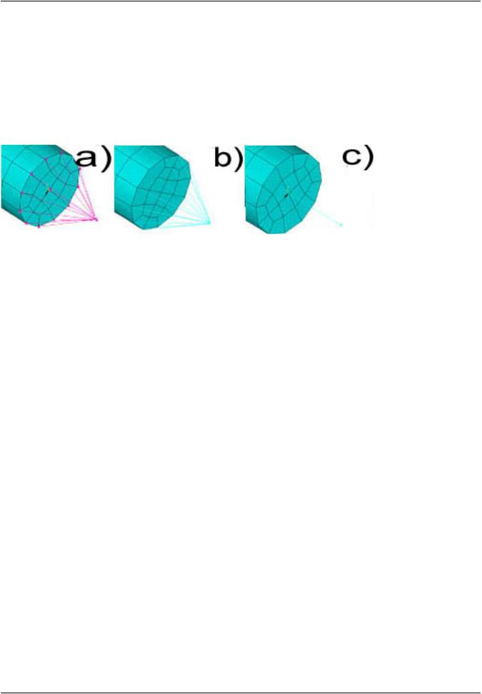
Figure 12.1: Connecting a Structure to an Interface Point (p. 318) shows three different ways that you may attempt to attach an interface point to a structure. The first two examples (a and b) demonstrate valid methods of attachment. The third example (c) demonstrates a poor method of attachment that should not be used.
Figure 12.1: Connecting a Structure to an Interface Point
Each method depicted in the figure is described below.
•a) Constraint equations are connecting the interface point to the structure. This method is recommended because:
–Force is distributed over an area.
–A MASS21 element is used to define the six degrees of freedom of the interface point.
–Moment loads are transmitted.
•b) A spider web of beams is connecting the interface point to the structure. This method is recommended (and preferred) because:
–Force is distributed over an area.
–No MASS21 element is necessary (because the beams supply the six degrees of freedom).
–Moment loads are transmitted.
• c) One beam is used to connect the interface point to the structure. This is not recommended because:
–The force is applied to the structure at a single node.
–Solid elements do not have rotational degrees of freedom. Therefore, moments will not be properly transmitted from the interface point to the structure (a spider web scheme should be used).
12.4. Exporting to ADAMS
After building the model in Mechanical APDL (including all interface points), the next step is to invoke the ANSYS-ADAMS Interface to create the modal neutral file, Jobname.MNF. Creation of this file is driven by a command macro called ADAMS.MAC.
To start the interface, select the following GUI path.
Main Menu> Solution> ADAMS Connection> Export to ADAMS
|
Release 15.0 - © SAS IP, Inc. All rights reserved. - Contains proprietary and confidential information |
318 |
of ANSYS, Inc. and its subsidiaries and affiliates. |
vk.com/club152685050 | vk.com/id446425943 |
Exporting to ADAMS |
The Select Interface Points dialog box appears first. From this dialog box, you must select two or more interface points.
Do not select too many interface points, as one point gives rise to six degrees of freedom in ADAMS. Too many interface points may lead to huge files and models.
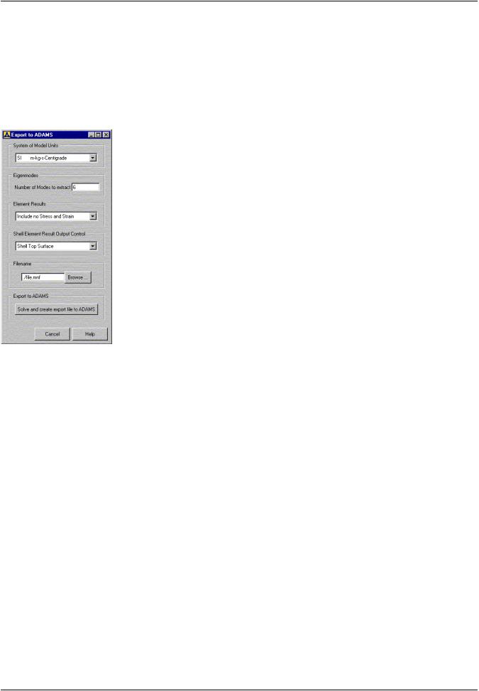
After you confirm your selection, the Export to ADAMS dialog box appears.
Figure 12.2: Export to ADAMS Dialog Box
Complete the following steps using this dialog box.
1.System of Model Units: The units used for the model is important to the ADAMS program, whereas Mechanical APDL only requires that you use a consistent set of units. The units chosen will be written to the .MNF file and can be recalled with the ADAMS/Flex module. If no units are specified, ADAMS assumes that the same units were used in Mechanical APDL as the ones chosen in the ADAMS model. See the /UNITS command for details. If you specify user defined units, a Define User Units dialog box will appear for you to input the conversion factors (for length, mass, force, and time) between SI units and
your chosen units. Below is an example of user defined units in which the component has been modeled using millimeter, tonne (metric ton), newton, and second.
Length Factor |
1 meter/milli- |
= |
= |
meter |
1000 |
Mass Factor = |
1 kilo- |
= |
|
gram/tonne |
0.001 |
Force Factor |
1 newton/new- |
= 1 |
= |
ton |
|
Time Factor = 1 second/second |
= 1 |
|
2.Number of Modes to Extract: Input the number of normal modes to compute. Normal modes are the eigenmodes of the component with all degrees of freedom of all interface points fixed. The number of normal modes depends on the frequency range of the excitation you will apply in your ADAMS model. You must select a sufficient number of modes to represent your structure in that frequency range. In
Release 15.0 - © SAS IP, Inc. All rights reserved. - Contains proprietary and confidential information |
|
of ANSYS, Inc. and its subsidiaries and affiliates. |
319 |

vk.com/club152685050Rigid-Body Dynamics and the| vkANSYS.com/id446425943-ADAMS Interface
ADAMS, if you have chosen too many normal modes, you are able to deactivate eigenmodes based on the frequency or an energy criterion.
3.Element Results: Specify whether or not the program should write stress and/or strain results. This option has no effect on the output for beam elements. If you want to output stress and strain for only a subset of nodes, you should create a node component named "STRESS" before running the ADAMS command macro.
4.Shell Element Result Output Control: Specify the shell element output location (top, middle, bottom). This option has no effect on the output for solid elements and beam elements.
5.Filename: Specify a filename for the modal neutral file. The default name is Jobname.MNF. If a file with the chosen name exists, it will be moved to a file named filename.MNFBAK.
6.Export to ADAMS: Select “Solve and create export file to ADAMS” to initiate the solution sequence. Static and normal modes are computed and all information required by ADAMS is written to the .MNF file specified above. Only the selected elements are considered. The current model is written to the database file Jobname.DBMNF.
Note
Note that the algorithm used to compute the .MNF file adds constraints to the interface points. If you create the .MNF file a second time using the same model in the same run, be sure to delete all constraints on the interface points (or resume the database file Jobname.DBMNF) before you run it again.
12.4.1. Exporting to ADAMS via Batch Mode
If you prefer to work in batch mode, you may choose to run the ADAMS command macro by command input. After building the model and defining interface points, use the following commands to compute the .MNF file.
/UNITS,Label |
! Specify the units chosen for |
modeling |
||||
NSEL,... |
! Select two or more |
interface |
points |
|||
SAVE |
! Save |
the |
model for |
a possible |
resume from |
|
|
! |
this |
point |
|
|
|
ADAMS,NMODES,... |
! |
Activate |
ADAMS.MAC |
to compute |
the .MNF file |
|
See the ADAMS command description for more information. When you use command input to compute the .MNF file, there is no option to change the file name. The default name of Jobname.MNF will be used.
12.4.2. Verifying the Results
It is a good practice to verify the correctness of the results after the .MNF file is created. Below are guidelines you can use to complete this task.
•Check the number of orthonormalized eigenmodes in the Mechanical APDL output window. These eigenmodes are the result of an orthonormalization of the normal modes and the constraint modes. You should observe the following:
– The number of modes equals the number of normal modes plus the number of constraint modes.
|
Release 15.0 - © SAS IP, Inc. All rights reserved. - Contains proprietary and confidential information |
320 |
of ANSYS, Inc. and its subsidiaries and affiliates. |