vk.com/club152685050 | vk.com/id446425943

Chapter 16: Soil-Pile-Structure Analysis

You can analyze the interaction of a structure, supported on one or more piles, with an elastic or inelastic soil. The analysis can take into account the lateral force-displacement, and the end-bearing and skinfriction responses, of the soil layers occurring at the pile location. It is not necessary for all piles in the analysis to be situated in identical geological strata.

Data input is defined primarily via the PILExxxx family of commands, with soil data defined in additional text files. Piles are connected to MATRIX27 elements which must be defined at the pile caps.

A number of codes of practice can be used to assess the strength of the piles.

The following soil-pile-structure analysis topics are available:

16.1.Soil-Pile-Structure Interaction Analysis

16.2.Soil Data Definition and Examples

16.3.Performing a Soil-Pile Interaction Analysis

16.4.Soil-Pile-Structure Results

16.5.References

16.1. Soil-Pile-Structure Interaction Analysis

MATRIX27 elements are used to locate the pile and to connect it to an above ground structure, or to apply loads directly for single pile only modeling. For pile stiffness modelling, use MATRIX27 element with KEYOPT(3) = 4. If pile mass is also required, another MATRIX27 element is required with KEYOPT(3) = 2. Each pile stiffness and mass element should be given a separate real constant number. The stiffness and/or mass values will be updated by issuing the relevant commands (PILEMASS, PILESTIF). The two nodes on the MATRIX27 stiffness element define the pile cap and pile tip position, respectively. The

pile cap node is the pile node that is connected to the supported structure.

The soil material properties must be specified on a layer by layer basis. For each stratum, the lateral force-displacement curve (P-Y curve) and the skin friction force-displacement curve (T-Z curve) may be input. For the lowest stratum the end-bearing force-displacement curve may also be defined. All of these three force-displacement relationships are piecewise linear curves with no restriction on the number of line segments allowed.

For the initial conditions the soil stiffness, as defined by the curves for zero displacement, is added to the pile stiffness and the displacements are calculated, assuming no change in the soil properties. These displacements are compared with the values at which the soil force-displacement curves become nonlinear. If the soil has become non-linear, that is the force-displacement relationship is no longer on the initial part of the curve, the soil stiffness is recalculated for the current displacement. The modified soil stiffness is added to the pile stiffness and a new set of displacements calculated. Iteration continues in this way until the displacements calculated in an iteration differ from those of the preceding iteration by less than a small tolerance.

These converged values of displacement are taken to be an adequate estimate of the true behavior. The program outputs the pile cap displacements and forces, and the pile’s displacements.

Unity checks may be requested against the following codes of practice:

vk.com/club152685050S il-Pile-Structure Analysis | vk.com/id446425943

•American Petroleum Institute (API) Recommended Practice for Planning, Designing and Constructing Fixed Offshore Platforms - Working Stress Design, RP2A-WSD, Twenty-first Edition, December 2000 (the Seventeenth and Twentieth editions are also supported).

•American Petroleum Institute (API) Recommended Practice for Planning, Designing and Constructing Fixed Offshore Platforms - Load and Resistance Factor Design, RP2A-LRFD, First Edition, July 1, 1993.

•International Standards Organization (ISO) 19902, Petroleum and Natural Gas Industries - Fixed Steel Offshore Structures, First Edition, December 2007.

In order to calculate these unity checks, yield data must be supplied for the piles. For WSD checks, extreme environmental loads may be specified.

For a transient analysis, the pile calculation should be calculated at each time step, in order for the updated loading (in the form of prescribed displacements) to be applied to the pile and a new stiffness and loading to be calculated and applied to the pile cap. In this case FDELE should be used to ensure that previously calculated nodal forces are not appended to.

Note

Multiple loadsteps and small time increments are necessary to allow for the nonlinear iterations required for the soil-pile interaction equations, and to enable these calculations to converge.

16.1.1. Automatic Pile Subdivision

Each pile is defined by two nodes on the MATRIX27 stiffness element. In order to calculate the structural stiffness of the pile and the soil to a sufficient degree of accuracy, the individual piles are automatically subdivided into a number of finite elements. Pile subdivisions will occur based on the following criteria:

1.The subdivision length will be related to the nominal diameter of the pile multiplied by a basic subdivision value (default 1.0) plus a percentage of the depth below the local mudline given by the subdivision modifier (default 0.1 or 10%). The depth used is taken at the mid-point of the existing subdivision. Both the basic subdivision value and the subdivision modifier may be specified in the PILEGEN command.

2.Each subdivision will be greater than 10% of the nominal pile diameter.

3.Whether there are any changes in the soil properties due to crossing from one stratum to another.

It is important to note that while the automatic subdivision process will provide a satisfactory result for general soil conditions, there are instances when user defined divisions are preferable. In particular, if only a few soil layers have been defined then the resultant subdivisions may prove to be too coarse and provide poor lateral displacements. It is suggested that the resultant subdivision information be inspected for large sub-elements in the critical top one third of the pile. As a rule of thumb, the subdivisions should be less than two times the pile diameter in the critical zone.

Item 2, above, prevents ill conditioning due to two closely spaced points occurring in the subdivision process. Where violation of this criterion occurs, the points are adjusted to be coincident. The program defined default cannot be amended.

16.1.2. Convergence Criteria

The analysis process is based upon the solution of the simultaneous equations relating to the pile caps and associated structural elements. Since, in general, the soil is of a nonlinear nature the solution

method utilizes an iterative technique whereby the soil stiffness and associated reactive loads are updated from the results of the previous iteration. Successive iterations modify the soil properties with progressively smaller resultant changes to the behavior of the pile model. In order that the analysis terminates within a finite number of iterations, a convergence tolerance is applied as follows:

•On the first iteration the pile cap displacements and reactions are calculated and stored.

•On the second and subsequent iterations, revised pile cap displacements and reactions are computed and compared with the previous iteration. If the percentage difference is greater than that defined (either

by program default or user input) the revised displacements are stored and the iteration process continued. The default convergence criteria is taken as 5%. This can be modified using the option in the PILEGEN command.

It is suggested that a lower limit of 0.1% for a single pile is observed in order to prevent an excessive number of iterations for convergence.

In addition to the convergence criteria described above, a simple divergence check is included in order to trap numerical instabilities introduced due to multiple pile failure or highly nonlinear systems. In some instances it may be desirable to switch this facility off using the ITER option on the PILEGEN command. It is suggested that this option is included only after reference to the iteration report confirms that no inherent instability exists.

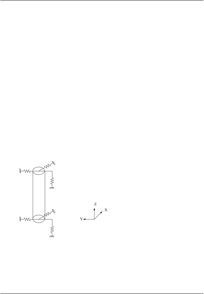
16.1.3. Soil Representation

The nonlinear foundation analysis method utilizes a finite element representation of the pile and soil system. Figure 16.1: Pile/Spring Foundation Model (p. 349) illustrates a typical element representing a pile segment and associated springs employed to model the soil.

Figure 16.1: Pile/Spring Foundation Model

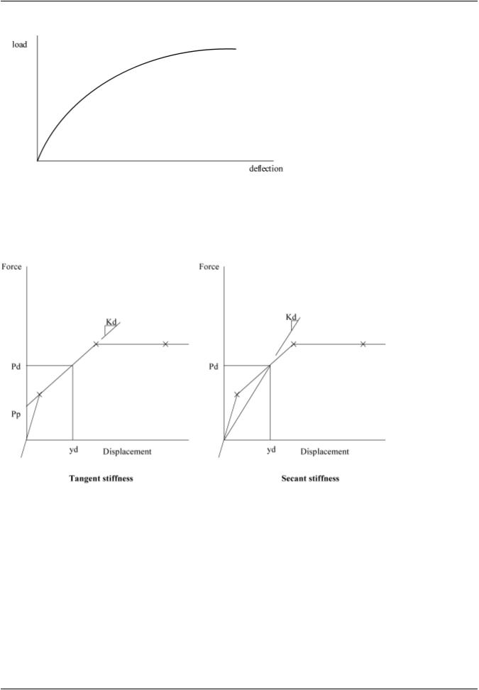
The springs utilized for the soil model are characterized by a nonlinear force-deflection relationship of the type shown in Figure 16.2: Soil/load Deflection Characteristics (p. 350). These are commonly known as P-Y curves for lateral behavior and T-Z curves for axial behavior.

vk.com/club152685050S il-Pile-Structure Analysis | vk.com/id446425943

Figure 16.2: Soil/load Deflection Characteristics

The nonlinear nature of the soil properties means an iterative solution technique is required. Each iteration takes an assumed, or calculated, value for the soil spring stiffness based upon the previous iteration.

Two solution methods exist for determining the representative soil stiffness from the defined P-Y and T-Z curves, namely Tangent and Secant stiffness. These are shown diagramatically below:

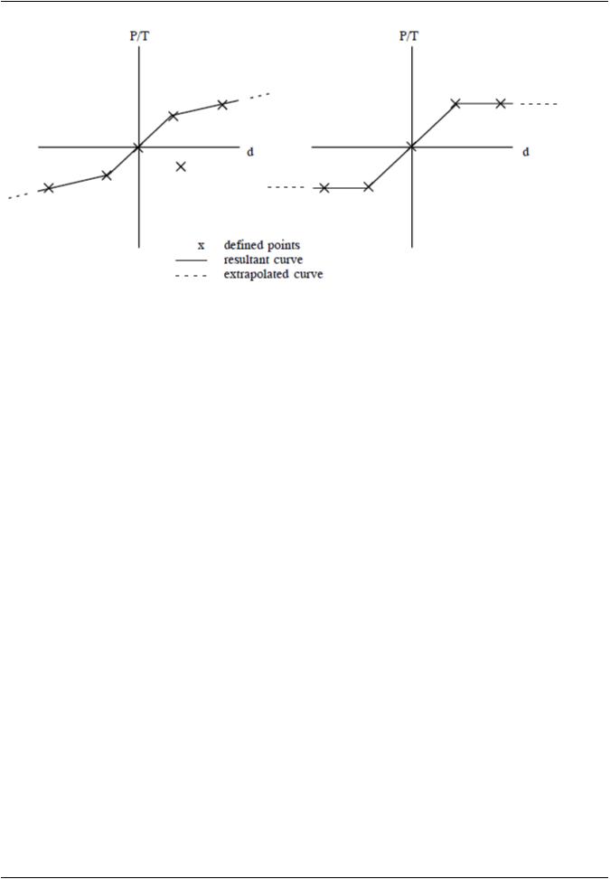
For both types of soil representation, the curves are stored as a series of points as defined by the user and depicted by crosses in the diagrams above. In order that the soil stiffness may be computed, the soil properties are assumed to vary linearly between these points as shown above. For points beyond the last y datum defined, linear extrapolation is utilized from the last two points supplied.

In general, the tangent stiffness method will converge faster than the secant stiffness approach, especially as the pile approaches its limiting capacity. The tangent stiffness method is adopted by default. The default may be overridden by the STIFF option in the PILEGEN command.

There is no limit to the number of points on any curve. For displacements that occur outside of the range specified for a given curve, linear extrapolation of the last segment of the curve is assumed. If a constant value is required, two points with similar P or T and different displacement must be input.

Both symmetric and non-symmetric curves may be defined for soil layer data. If symmetric curves are required, only that part of the curve for positive displacement values need be input. The program will automatically generate the remaining information.

If any values are defined for a negative displacement, then the curve is assumed to be non-symmetric. Care should be taken in providing non-symmetric P-Y data since the soil stiffnesses derived from the curves are based upon local axes displacements, and these may vary from pile to pile and from iteration to iteration. Shifted P-Y curves are not permitted, since this can result in undesired lateral deflections. Use the SLID definition if shifted curves are required.

For T-Z and ENDB data, a positive local displacement for the purposes of soil stiffness formulation is taken as being defined by the vector going from the pile cap to the pile tip. Thus, zero tensile stiffness for end bearing forces may be modelled by supplying an ENDB definition with zero stiffness for negative displacements.

The soil properties must be defined down to the full depth of the pile, or to a greater depth.

If both top and bottom layer depths are supplied on a P-Y or T-Z header, the data is taken as a constant between these depths. If only one depth is supplied, the data is defining the properties at one depth

in the soil medium. P-Y and T-Z curves, either explicitly defined or generated from the soil properties, are assumed to vary linearly between these depths.

If a sudden change in soil properties is required at a given depth, one of two options are available:

1.If one or both of the soil definitions represent a constant stratum, the given depth may be supplied for both layers.

2.If both the soil definitions are single point, they must be separated by a finite distance so that the program

can identify which layer is uppermost. Provided the separation is less than the coordinate tolerance (0.1 x pile diameter) the program will utilize the data as though they represented coincident layers. The higher of the two levels specified will be adopted as the point of the discontinuity. See also Automatic Pile Subdivision (p. 348).

vk.com/club152685050S il-Pile-Structure Analysis | vk.com/id446425943

The procedures used for developing P-Y and T-Z curves from user defined soil properties are as indicated in the list below. Detailed descriptions are not given but a typical curve for each procedure is shown.

Note

Overburden pressures used in the soil curve generation are computed from the soil densities provided down the soil profile. If explicit P-Y and/or T-Z data is provided for any soil layer within a soil profile, then overburden pressures will be computed based upon the soil density local to the point of calculation.

The α factor used for shaft friction is automatically calculated as specified in Clause 6.4.2 of the API 21st edition. A limiting value of ϕ is set to 3.0. However no allowance is made for pile length.

The resulting soil curves depend upon the pile to which it is to be applied since, in the general form, pressures are generated. A different soil curve set will thus be produced for each pile in an analysis. Where stepped piles are utilized, it is important that two soil definitions are provided at the step position(s) in order that the correct geometric data is utilized for the curve generation.

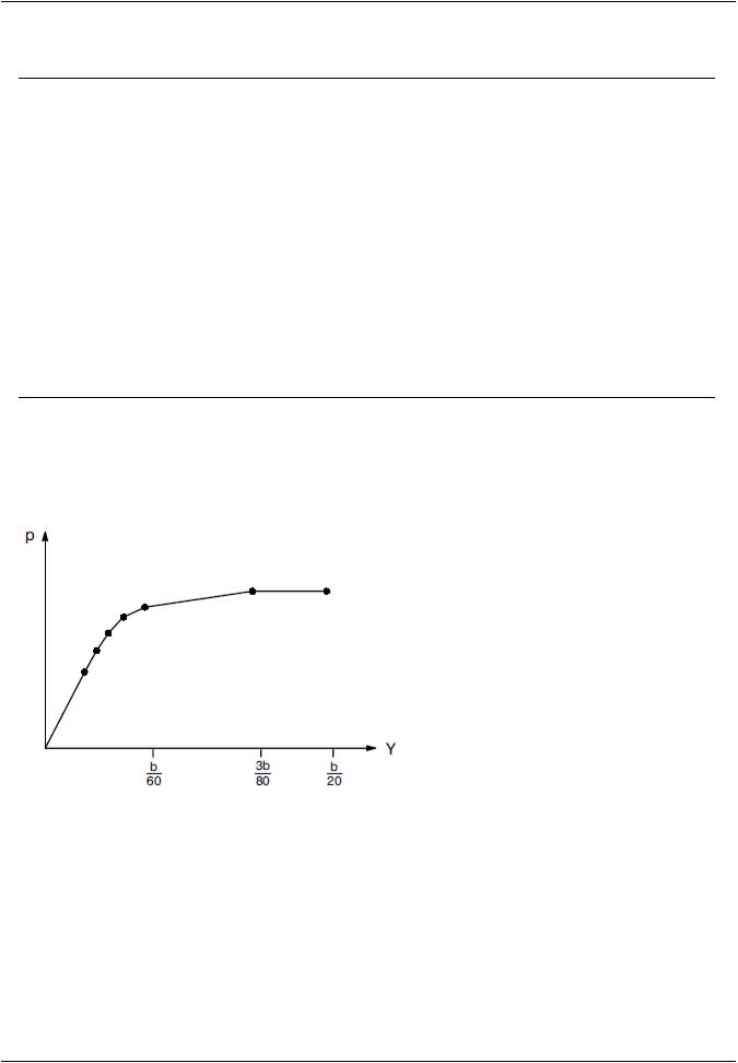
Procedures for Developing P-Y and T-Z Curves

•For sands, the method suggested by Reese, et. al. [1] is used.

Figure 16.3: P-Y Curve for Sand

•For clays, the method suggested by Matlock [2], a modified Matlock procedure, and the basic recommendations as listed in API 15 [3] are available.

Figure 16.4: P-Y Curve for Clay: Static Loading

Figure 16.5: P-Y Curve for Clay: Cyclic Loading

•For T-Z and ENDB curves, the procedures recommended by Vijayvergiya [4] have been adopted.

For the purposes of the implementation in the ANSYS soil-pile analysis, the ultimate skin friction and end bearing pressure that can be developed in cohesionless soils (sand) is limited to the values given in the API RP2A code of practice. The user should also note that for plugged pile conditions it is assumed that any internal soil skin friction is sufficient to sustain the plug in position; there is no internal check undertaken to check this requirement.