vk.com/club152685050Rezoning | vk.com/id446425943

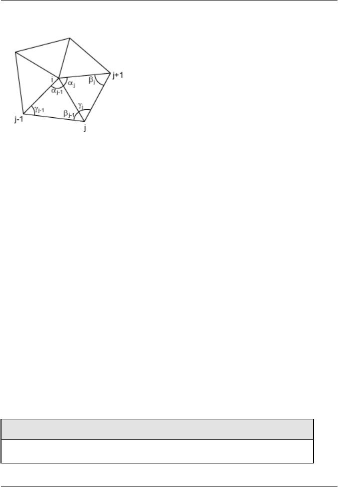
Figure 4.14: Mesh Morphing Using Cotangent-Weighted Laplacian Equation

The mesh-morphing process stops when the node movement no longer improves shape metrics or the magnitude of the node movement becomes negligibly small.

4.7.2. Mesh Control

Creating a better mesh is the key to successful rezoning. The new mesh must be better than the old mesh; otherwise, rezoning cannot improve convergence, and can even result in nonconvergence if the new mesh is worse.

Generally, a good mesh has these characteristics:

•The element internal angles do not approach 180 degrees or 0 degrees.

•The opposite edges or faces of quadrilaterals have less cross angle (that is, they are closer to parallel with each other).

•Boundary nodes are more evenly distributed.

•The elements have a better aspect ratio.

For creating a good mesh, satisfactory internal angles are a more important consideration than whether aspect ratios may be too high or too low. For 2-D meshes, avoid triangle elements as much as possible; however, if quadrilateral elements have very large internal angles, it is preferable to accept some triangle elements with more acceptable internal angles instead.

The quality of the new mesh is fully dependent on the shape of the selected region, neighboring elements, and boundary nodes with applied loads and boundary conditions. It may sometimes be necessary to edit or modify the new mesh prior to the mapping operation (MAPSOLVE); in such cases, several preprocessing (/PREP7) commands are available to help you create a good mesh on the selected region:

Figure 4.15: /PREP7 Mesh-Control Commands Available in Rezoning

Type of Mesh ConApplicable Commands trol Desired

Type of Mesh ConApplicable Commands trol Desired

Boundary node disBoundary nodes require special attention. Use the LESIZE command to

The mesh-control commands are available at any point after issuing a REMESH,START command and before issuing a REMESH,FINISH command.

Nodes at which force or isolated displacements are applied must remain during remeshing, as do nodes at the boundaries of distributed displacements, pressures, or contact/target surfaces. The new elements must have the same attributes as the old elements, such as element type, material, real constant, and element coordinate system. The program rotates the new nodes to the same angles as the old nodes

in the region or on the boundary, as the case may be.

After creating the new mesh, verify that the new elements cover the entire selected region and are compatible with neighboring regions. (If another region requires remeshing, you can do so, but do not issue another REMESH,START command.

4.7.3. Remeshing Multiple Regions at the Same Substep

You can create a new mesh for more than one region in the same deformed domain. Remeshing two or more regions at the same specified substep is called horizontal rezoning.

You must use horizontal rezoning if you intend to remesh:

•Two regions with different materials, element coordinate systems, nodal coordinate systems, or real constants.

•The elements on both sides of a contact boundary.

•Two groups of highly distorted, noncontiguous elements.

Horizontal rezoning using a program-generated new mesh or a generic new mesh is possible only when the remeshed areas are isolated from each other or, at most, share an interface; however, the remeshed areas may not intersect. This restriction does not exist for manual mesh splitting.