1.5. Probabilistic Design Techniques

Understanding the algorithm used by a computer program is always helpful; this is particularly true in the case of probabilistic design. This section presents details on the method types and the sampling options associated with each. See the Mechanical APDL Theory Reference for more information.

1.5.1. Monte Carlo Simulations

The Monte Carlo Simulation method is the most common and traditional method for a probabilistic analysis. This method lets you simulate how virtual components behave the way they are built. One simulation loop represents one manufactured component that is subjected to a particular set of loads and boundary conditions.

For Monte Carlo simulations, you can employ either the Direct Sampling method or the Latin Hypercube Sampling method.

When you manufacture a component, you can measure its geometry and all of its material properties (although typically, the latter is not done because this can destroy the component). In the same sense, if you started operating the component then you could measure the loads it is subjected to. Again, to actually measure the loads is very often impractical. But the bottom line is that once you have a component in your hand and start using it then all the input parameters have very specific values that you

could actually measure. With the next component you manufacture you can do the same; if you compared the parameters of that part with the previous part, you would find that they vary slightly. This comparison of one component to the next illustrates the scatter of the input parameters. The Monte Carlo Simulation techniques mimic this process. With this method you “virtually” manufacture and operate components or parts one after the other.

The advantages of the Monte Carlo Simulation method are:

•The method is always applicable regardless of the physical effect modeled in a finite element analysis. It not based on assumptions related to the random output parameters that if satisfied would speed things up and if violated would invalidate the results of the probabilistic analysis. Assuming the deterministic model is correct and a very large number of simulation loops are performed, then Monte

Carlo techniques always provide correct probabilistic results. Of course, it is not feasible to run an infinite number of simulation loops; therefore, the only assumption here is that the limited number of simulation loops is statistically representative and sufficient for the probabilistic results that are evaluated. This assumption can be verified using the confidence limits, which the PDS also provides.

•Because of the reason mentioned above, Monte Carlo Simulations are the only probabilistic methods suitable for benchmarking and validation purposes.

•The individual simulation loops are inherently independent; the individual simulation loops do not depend on the results of any other simulation loops. This makes Monte Carlo Simulation techniques ideal candidates for parallel processing.

The Direct Sampling Monte Carlo technique has one drawback: it is not very efficient in terms of required number of simulation loops.

1.5.1.1. Direct Sampling

Direct Monte Carlo Sampling is the most common and traditional form of a Monte Carlo analysis. It is popular because it mimics natural processes that everybody can observe or imagine and is therefore easy to understand. For this method, you simulate how your components behave based on the way

vk.com/club152685050Probabi istic Design | vk.com/id446425943

they are built. One simulation loop represents one component that is subjected to a particular set of loads and boundary conditions.

The Direct Monte Carlo Sampling technique is not the most efficient technique, but it is still widely used and accepted, especially for benchmarking and validating probabilistic results. However, benchmarking and validating requires many simulation loops, which is not always feasible. This sampling method is also inefficient due to the fact that the sampling process has no "memory."

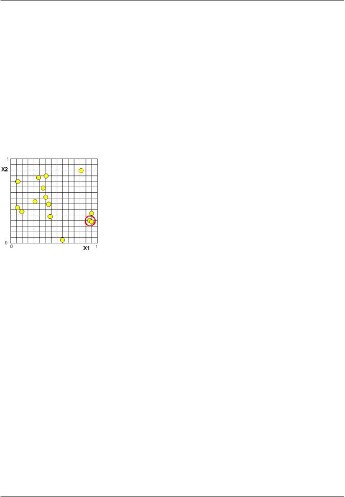
For example, if we have two random input variables X1 and X2 both having a uniform distribution ranging from 0.0 to 1.0, and we generate 15 samples, we could get a cluster of two (or even more) sampling points that occur close to each other if we graphed the two variables (see figure below). While in the space of all random input variables, it can happen that one sample has input values close to another sample, this does not provide new information and insight into the behavior of a component in a computer simulation if the same (or almost the same) samples are repeated.

Figure 1.7: Graph of X1 and X2 Showing Two Samples with Close Values

To use Direct Monte Carlo Sampling, do the following

Command(s): PDMETH,MCS,DIR PDDMCS

GUI: Main Menu> Prob Design> Prob Method> Monte Carlo Sims

In this sampling method, you set the number of simulations, whether to stop simulations loops when certain criteria are met (accuracy for mean values and standard deviations), and the seed value for randomizing input variable sample data.

1.5.1.2. Latin Hypercube Sampling

The Latin Hypercube Sampling (LHS) technique is a more advanced and efficient form for Monte Carlo Simulation methods. The only difference between LHS and the Direct Monte Carlo Sampling technique is that LHS has a sample "memory," meaning it avoids repeating samples that have been evaluated

before (it avoids clustering samples). It also forces the tails of a distribution to participate in the sampling process. Generally, the Latin Hypercube Sampling technique requires 20% to 40% fewer simulations loops than the Direct Monte Carlo Simulation technique to deliver the same results with the same accuracy. However, that number is largely problem dependent.

Figure 1.8: Graph of X1 and X2 Showing Good Sample Distribution

To use the Latin Hypercube Sampling technique:

Command(s): PDMETH,MCS,LHS PDLHS

GUI: Main Menu> Prob Design> Prob Method> Monte Carlo Sims

In this sampling method, you set the number of simulations and repetitions, the location in the interval for the sample, whether the simulations stop when certain criteria are met (accuracy of mean values and standard deviations), and random number seed for variability in the sample input variable data.

1.5.1.3. User-Defined Sampling

For this method, you provide the file containing the samples.

Command(s): PDMETH,MCS,USER PDUSER

GUI: Main Menu> Prob Design> Prob Method> Monte Carlo Sims

By using this option you have complete control over the sampling data. You are required to give the file name and path.

If user-specified sampling methods are requested with the PDMETH,MCS,USER command or the PDMETH,RSM,USER command, then you need to specify which file contains the sample data. The sample data is a matrix, where the number of columns is equal to the number of defined random variables and the number of lines is equal to the number of simulation loops requested. This data must be contained in an ASCII file and the content must obey the following notations and format requirements:

•Column separators allowed: blank spaces, commas, semicolons, and tabs.

•Multiple blank spaces and multiple tabs placed directly one after the other are allowed and are considered as one single column separator.

•Multiple commas or semicolons placed directly one after the other are not allowed; for example, two commas with no data between them (just blanks) are read as an empty column, which leads to an error message.

•The first line of the file must contain a solution label. No additional data is allowed on the first line, and if found, will lead to an error message. An error message is also issued if the solution label is missing.

•The solution label is just a placeholder. For consistency, you should use the same solution label you specify in the PDEXE command, but if they are different, you will always use the solution label specified

vk.com/club152685050Probabi istic Design | vk.com/id446425943

in the PDEXE command for postprocessing. The PDS system does not check if the solution label in the user-specified file and the one given in the PDEXE command match.

•The second line of the file must contain the headers of the data columns. The first three column headers must be “ITER”, “CYCL”, and “LOOP”, respectively; then subsequent columns should contain the names of the random variables. You must use one of the allowed separators as described above between the column headers. No additional data is allowed on this line, and if found, will prompt an error message. An error message is also issued if any of the required column headers are missing.

•The random variable names in your file must match the names of the defined random variables. The variable names that you specify must consist of all uppercase characters (regardless of the case used in the defined variable names).

•Columns four to n can be in arbitrary order. The ANSYS PDS tool determines the order for the random variable data based on the order of the random variable names in the second line.

•The third and subsequent lines must contain the order number for the iteration, cycle, and simulation loop, then the random variable values for that loop. The iteration, cycle, and simulation loop numbers must be in the first, second, and third columns respectively, followed by the random variable values.

The iteration and cycle numbers are used by the ANSYS PDS (internally) and for a user-defined sampling method you will typically use a value of "1" for all simulation loops. The loop number is an ascending number from 1 to the total number of loops requested. Additional data is not allowed, and if found, will lead to an error message. An error message is also issued if any of the data columns are missing.

•You must be sure that the order of the random variable values in each line is identical to the order of the random variable names in the second line.

•The user-specified sampling file must contain a minimum of one data line for the random variable values.

When the PDUSER command is issued, the PDS checks that the specified file exists, then verifies it for completeness and consistency. Consistency is checked according to the possible minimum and maximum boundaries of the distribution type of the individual random variables. An error message is issued if a random variable value is found in the file that is below the minimum boundary or above the maximum boundary of the distribution of that random variable. This also means that any value will be accepted

for a random variable if its distribution has no minimum or maximum boundary; for example, this is the case for the Gaussian (normal) distribution. Apart from this check, it is your responsibility to provide values for the random variables that are consistent with their random distribution.

Note

It is your responsibility to ensure that parameters defined as random input variables are actually input parameters for the analysis defined with the PDANL command. Likewise, you

must ensure that parameters defined as random output parameter are in fact results generated in the analysis file.

Example

An excerpt of the content of a user-specified sampling file is given below. This example is based on three random variables named X1, X2, and X3. A total of 100 simulation loops are requested.