•Retrieve and assign to parameters the quantities that will be used as random input variables and random output parameters (POST1/POST26).

2.Establish parameters in the database which correspond to those used in the analysis file. This step is typical, but not required (Begin or PDS); however, if you skip this step, then the parameter names are not available for selection in interactive mode.

3.Enter PDS and specify the analysis file (PDS).

4.Declare random input variables (PDS).

5.Visualize random input variables (PDS). Optional.

6.Specify any correlations between the RVs (PDS).

7.Specify random output parameters (PDS).

8.Select the probabilistic design tool or method (PDS).

9.Execute the loops required for the probabilistic design analysis (PDS).

10.Fit the response surfaces (if you did not use a Monte Carlo Simulation method) (PDS).

11.Review the results of the probabilistic analysis (PDS).

Because analyzing complex problems can be time-consuming, you have the option of running a probabilistic analysis on a single processor or distributing the analyses across multiple processors. By using the PDS parallel-run capabilities, you can run many analysis loops simultaneously and reduce the overall run time for a probabilistic analysis.

1.3.1. Create the Analysis File

The analysis file is crucial to probabilistic design. The probabilistic design system (PDS) uses the analysis file to form the loop file, which in turn is used to perform analysis loops. Any type of analysis (structural, thermal, magnetic, etc.; linear or nonlinear) may be incorporated into the analysis file.

The model must be defined in terms of parameters (both RVs and RPs). Only numerical scalar parameters are used by the PDS. See Use ANSYS Parameters in the Modeling and Meshing Guide for a discussion of parameters. See the ANSYS Parametric Design Language Guide for a discussion of the ANSYS Parametric Design Language (APDL).

It is your responsibility to create and verify the analysis file. It must represent a clean analysis that will run from start to finish. Most nonessential commands (such as those that perform graphic displays, listings, status requests, etc.) should be stripped off or commented out of the file. Maintain only those display commands that you want to see during an interactive session (such as EPLOT), or direct desired displays to a graphics file (/SHOW). Because the analysis file will be used iteratively during probabilistic design looping, any commands not essential to the analysis will decrease efficiency.

You can create an analysis file by inputting commands line by line via a system editor, or you can create the analysis interactively in the program and use the command log as the basis for the analysis file.

Creating the file with a system editor is the same as creating a batch input file for the analysis. (If you are performing the entire probabilistic design in batch mode, the analysis file is usually the first portion of the complete batch input stream.) This method allows you full control of parametric definitions through exact command inputs. It also eliminates the need to clean out unnecessary commands later.

vk.com/club152685050Probabi istic Design | vk.com/id446425943

You prefer to perform the initial analysis interactively, and then use the resulting command log as the basis for the analysis file. In this case, you must edit the log file to make it suitable for probabilistic design looping. For more information about using the log files, see Using the ANSYS Session and Command Logs in the Operations Guide.

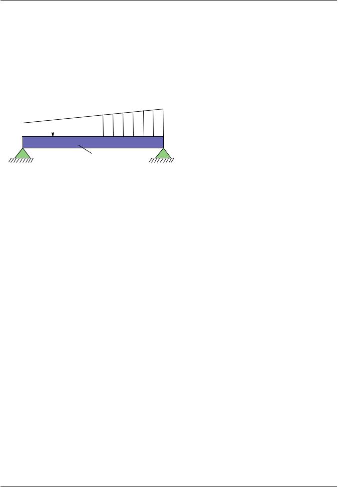
1.3.1.1. Example Problem Description

The simple beam problem introduced earlier illustrates a probabilistic design analysis.

Figure 1.3: A Beam Under a Snow Load

H1 H2

E

Young's modulus is 20E4.

1.3.1.2. Build the Model Parametrically

PREP7 is used to build the model in terms of the RV parameters. For our beam example, the RV parameters are H1 (snow height at left end), H2 (snow height at right end), and the Young's modulus E.

...

!Initialize parameters:

As mentioned earlier, you can vary virtually any aspect of the design: dimensions, shape, material property, support placement, applied loads, etc. The only requirement is that the design be defined in

terms of parameters. The RV parameters (H1, H2, and E in this example) may be initialized anywhere, but are typically defined in PREP7.

Caution

If you build your model interactively (through the GUI), you will encounter many situations where data can be input through graphical picking (such as when defining geometric entities). Because some picking operations do not allow parametric input (and PDS requires parametric input), you should avoid picking operations. Instead, use menu options that allow direct input of parameters.

1.3.1.3. Obtain the Solution

The SOLUTION processor is used to define the analysis type and analysis options, apply loads, specify load step options, and initiate the finite element solution. All data required for the analysis should be specified: appropriate convergence criteria for nonlinear analyses, frequency range for analysis, and so on. Loads and boundary conditions may also be RVs as illustrated for the beam example here.

The SOLUTION input for our beam example could look like this:

This step is not limited to just one analysis. You can, for instance, obtain a thermal solution and then obtain a stress solution (for thermal stress calculations).

If your solution uses the multiframe restart feature, all changes to the parameter set that are made after the first load step will be lost in a multiframe restart. To ensure that the correct parameters are used

in a multiframe restart, you must explicitly save (PARSAV) and resume (PARESU) the parameters for use in the restart. See the Basic Analysis Guide for more information on multiframe restarts.

1.3.1.4. Retrieve Results and Assign as Output Parameters

This is where you retrieve results data and assign them to random output parameters to be used for the probabilistic portion of the analysis. Use the *GET command (Utility Menu> Parameters> Get Scalar Data), which assigns program-calculated values to parameters, to retrieve the data. POST1 is typically used for this step, especially if the data are to be stored, summed, or otherwise manipulated.