

- •Table of Contents
- •Chapter 1: Probabilistic Design
- •1.1. Understanding Probabilistic Design
- •1.1.1. Traditional (Deterministic) vs. Probabilistic Design Analysis Methods
- •1.1.2. Reliability and Quality Issues
- •1.2. Probabilistic Design Terminology
- •1.3. Using Probabilistic Design
- •1.3.1. Create the Analysis File
- •1.3.1.1. Example Problem Description
- •1.3.1.2. Build the Model Parametrically
- •1.3.1.3. Obtain the Solution
- •1.3.1.4. Retrieve Results and Assign as Output Parameters
- •1.3.1.5. Prepare the Analysis File
- •1.3.2. Establish Parameters for Probabilistic Design Analysis
- •1.3.3. Enter the PDS and Specify the Analysis File
- •1.3.4. Declare Random Input Variables
- •1.3.5. Visualize Random Input Variables
- •1.3.6. Specify Correlations Between Random Variables
- •1.3.7. Specify Random Output Parameters
- •1.3.8. Select a Probabilistic Design Method
- •1.3.8.1. Probabilistic Method Determination Wizard
- •1.3.9. Execute Probabilistic Analysis Simulation Loops
- •1.3.9.1. Probabilistic Design Looping
- •1.3.9.2. Serial Analysis Runs
- •1.3.9.3. PDS Parallel Analysis Runs
- •1.3.9.3.1. Machine Configurations
- •1.3.9.3.1.1. Choosing Slave Machines
- •1.3.9.3.1.2. Using the Remote Shell Option
- •1.3.9.3.1.3. Using the Connection Port Option
- •1.3.9.3.1.4. Configuring the Master Machine
- •1.3.9.3.1.5. Host setup using port option
- •1.3.9.3.1.6. Host and Product selection for a particular analysis
- •1.3.9.3.2. Files Needed for Parallel Run
- •1.3.9.3.3. Controlling Server Processes
- •1.3.9.3.4. Initiate Parallel Run
- •1.3.10. Fit and Use Response Surfaces
- •1.3.10.1. About Response Surface Sets
- •1.3.10.2. Fitting a Response Surface
- •1.3.10.3. Plotting a Response Surface
- •1.3.10.4. Printing a Response Surface
- •1.3.10.5. Generating Monte Carlo Simulation Samples on the Response Surfaces
- •1.3.11. Review Results Data
- •1.3.11.1. Viewing Statistics
- •1.3.11.2. Viewing Trends
- •1.3.11.3. Creating Reports
- •1.4. Guidelines for Selecting Probabilistic Design Variables
- •1.4.1. Choosing and Defining Random Input Variables
- •1.4.1.1. Random Input Variables for Monte Carlo Simulations
- •1.4.1.2. Random Input Variables for Response Surface Analyses
- •1.4.1.3. Choosing a Distribution for a Random Variable
- •1.4.1.3.1. Measured Data
- •1.4.1.3.2. Mean Values, Standard Deviation, Exceedence Values
- •1.4.1.3.3. No Data
- •1.4.1.4. Distribution Functions
- •1.4.2. Choosing Random Output Parameters
- •1.5. Probabilistic Design Techniques
- •1.5.1. Monte Carlo Simulations
- •1.5.1.1. Direct Sampling
- •1.5.1.2. Latin Hypercube Sampling
- •1.5.1.3. User-Defined Sampling
- •1.5.2. Response Surface Analysis Methods
- •1.5.2.1. Central Composite Design Sampling
- •1.5.2.2. Box-Behnken Matrix Sampling
- •1.5.2.3. User-Defined Sampling
- •1.6. Postprocessing Probabilistic Analysis Results
- •1.6.1. Statistical Postprocessing
- •1.6.1.1. Sample History
- •1.6.1.2. Histogram
- •1.6.1.3. Cumulative Distribution Function
- •1.6.1.4. Print Probabilities
- •1.6.1.5. Print Inverse Probabilities
- •1.6.2. Trend Postprocessing
- •1.6.2.1. Sensitivities
- •1.6.2.2. Scatter Plots
- •1.6.2.3. Correlation Matrix
- •1.6.3. Generating an HTML Report
- •1.7. Multiple Probabilistic Design Executions
- •1.7.1. Saving the Probabilistic Design Database
- •1.7.2. Restarting a Probabilistic Design Analysis
- •1.7.3. Clearing the Probabilistic Design Database
- •1.8. Example Probabilistic Design Analysis
- •1.8.1. Problem Description
- •1.8.2. Problem Specifications
- •1.8.2.1. Problem Sketch
- •1.8.3. Using a Batch File for the Analysis
- •1.8.4. Using the GUI for the PDS Analysis
- •Chapter 2: Variational Technology
- •2.1. Harmonic Sweep Using VT Accelerator
- •2.1.1. Structural Elements Supporting Frequency-Dependent Properties
- •2.1.2. Harmonic Sweep for Structural Analysis with Frequency-Dependent Material Properties
- •2.1.2.1. Beam Example
- •Chapter 3: Adaptive Meshing
- •3.1. Prerequisites for Adaptive Meshing
- •3.2. Employing Adaptive Meshing
- •3.3. Modifying the Adaptive Meshing Process
- •3.3.1. Selective Adaptivity
- •3.3.2. Customizing the ADAPT Macro with User Subroutines
- •3.3.2.1. Creating a Custom Meshing Subroutine (ADAPTMSH.MAC)
- •3.3.2.2. Creating a Custom Subroutine for Boundary Conditions (ADAPTBC.MAC)
- •3.3.2.3. Creating a Custom Solution Subroutine (ADAPTSOL.MAC)
- •3.3.2.4. Some Further Comments on Custom Subroutines
- •3.3.3. Customizing the ADAPT Macro (UADAPT.MAC)
- •3.4. Adaptive Meshing Hints and Comments
- •3.5. Where to Find Examples
- •Chapter 4: Rezoning
- •4.1. Benefits and Limitations of Rezoning
- •4.1.1. Rezoning Limitations
- •4.2. Rezoning Requirements
- •4.3. Understanding the Rezoning Process
- •4.3.1. Overview of the Rezoning Process Flow
- •4.3.2. Key Commands Used in Rezoning
- •4.4. Step 1: Determine the Substep to Initiate Rezoning
- •4.5. Step 2. Initiate Rezoning
- •4.6. Step 3: Select a Region to Remesh
- •4.7. Step 4: Perform the Remeshing Operation
- •4.7.1. Choosing a Remeshing Method
- •4.7.1.1. Remeshing Using a Program-Generated New Mesh (2-D)
- •4.7.1.1.1. Creating an Area to Remesh
- •4.7.1.1.2. Using Nodes From the Old Mesh
- •4.7.1.1.3. Hints for Remeshing Multiple Regions
- •4.7.1.1.4. Generating a New Mesh
- •4.7.1.2. Remeshing Using a Generic New Mesh (2-D and 3-D)
- •4.7.1.2.1. Using the REMESH Command with a Generic New Mesh
- •4.7.1.2.2. Requirements for the Generic New Mesh
- •4.7.1.2.3. Using the REGE and KEEP Remeshing Options
- •4.7.1.3. Remeshing Using Manual Mesh Splitting (2-D and 3-D)
- •4.7.1.3.1. Understanding Mesh Splitting
- •4.7.1.3.2. Geometry Details for Mesh Splitting
- •4.7.1.3.3. Using the REMESH Command for Mesh Splitting
- •4.7.1.3.4. Mesh-Transition Options for 2-D Mesh Splitting
- •4.7.1.3.5. Mesh-Transition Options for 3-D Mesh Splitting
- •4.7.1.3.7. Improving Tetrahedral Element Quality via Mesh Morphing
- •4.7.2. Mesh Control
- •4.7.3. Remeshing Multiple Regions at the Same Substep
- •4.8. Step 5: Verify Applied Contact Boundaries, Surface-Effect Elements, Loads, and Boundary Conditions
- •4.8.1. Contact Boundaries
- •4.8.2. Surface-Effect Elements
- •4.8.3. Pressure and Contiguous Displacements
- •4.8.4. Forces and Isolated Applied Displacements
- •4.8.5. Nodal Temperatures
- •4.8.6. Other Boundary Conditions and Loads
- •4.9. Step 6: Automatically Map Variables and Balance Residuals
- •4.9.1. Mapping Solution Variables
- •4.9.2. Balancing Residual Forces
- •4.9.3. Interpreting Mapped Results
- •4.9.4. Handling Convergence Difficulties
- •4.10. Step 7: Perform a Multiframe Restart
- •4.11. Repeating the Rezoning Process if Necessary
- •4.11.1. File Structures for Repeated Rezonings
- •4.12. Postprocessing Rezoning Results
- •4.12.1. The Database Postprocessor
- •4.12.1.1. Listing the Rezoning Results File Summary
- •4.12.1.2. Animating the Rezoning Results
- •4.12.1.3. Using the Results Viewer for Rezoning
- •4.12.2. The Time-History Postprocessor
- •4.13. Rezoning Restrictions
- •4.14. Rezoning Examples
- •4.14.1. Example: Rezoning Using a Program-Generated New Mesh
- •4.14.1.1. Initial Input for the Analysis
- •4.14.1.2. Rezoning Input for the Analysis
- •4.14.2. Example: Rezoning Using a Generic New Mesh
- •4.14.2.1. Initial Input for the Analysis
- •4.14.2.2. Exporting the Distorted Mesh as a CDB File
- •4.14.2.3. Importing the File into ANSYS ICEM CFD and Generating a New Mesh
- •4.14.2.4. Rezoning Using the New CDB Mesh
- •Chapter 5: Mesh Nonlinear Adaptivity
- •5.1. Mesh Nonlinear Adaptivity Benefits, Limitations and Requirements
- •5.1.1. Rubber Seal Simulation
- •5.1.2. Crack Simulation
- •5.2. Understanding the Mesh Nonlinear Adaptivity Process
- •5.2.1. Checking Nonlinear Adaptivity Criteria
- •5.2.1.1. Defining Element Components
- •5.2.1.2. Defining Nonlinear Adaptivity Criteria
- •5.2.1.3. Defining Criteria-Checking Frequency
- •5.3. Mesh Nonlinear Adaptivity Criteria
- •5.3.1. Energy-Based
- •5.3.2. Position-Based
- •5.3.3. Contact-Based
- •5.3.4. Frequency of Criteria Checking
- •5.4. How a New Mesh Is Generated
- •5.5. Convergence at Substeps with the New Mesh
- •5.6. Controlling Mesh Nonlinear Adaptivity
- •5.7. Postprocessing Mesh Nonlinear Adaptivity Results
- •5.8. Mesh Nonlinear Adaptivity Examples
- •5.8.1. Example: Rubber Seal Simulation
- •5.8.2. Example: Crack Simulation
- •Chapter 6: 2-D to 3-D Analysis
- •6.1. Benefits of 2-D to 3-D Analysis
- •6.2. Requirements for a 2-D to 3-D Analysis
- •6.3. Overview of the 2-D to 3-D Analysis Process
- •6.3.1. Overview of the 2-D to 3-D Analysis Process Flow
- •6.3.2. Key Commands Used in 2-D to 3-D Analysis
- •6.4. Performing a 2-D to 3-D Analysis
- •6.4.1. Step 1: Determine the Substep to Initiate
- •6.4.2. Step 2: Initiate the 2-D to 3-D Analysis
- •6.4.3. Step 3: Extrude the 2-D Mesh to the New 3-D Mesh
- •6.4.4. Step 4: Map Solution Variables from 2-D to 3-D Mesh
- •6.4.5. Step 5: Perform an Initial-State-Based 3-D Analysis
- •6.5. 2-D to 3-D Analysis Restrictions
- •Chapter 7: Cyclic Symmetry Analysis
- •7.1. Understanding Cyclic Symmetry Analysis
- •7.1.1. How the Program Automates a Cyclic Symmetry Analysis
- •7.1.2. Commands Used in a Cyclic Symmetry Analysis
- •7.2. Cyclic Modeling
- •7.2.1. The Basic Sector
- •7.2.2. Edge Component Pairs
- •7.2.2.1. CYCOPT Auto Detection Tolerance Adjustments for Difficult Cases
- •7.2.2.2. Identical vs. Dissimilar Edge Node Patterns
- •7.2.2.3. Unmatched Nodes on Edge-Component Pairs
- •7.2.2.4. Identifying Matching Node Pairs
- •7.2.3. Modeling Limitations
- •7.2.4. Model Verification (Preprocessing)
- •7.3. Solving a Cyclic Symmetry Analysis
- •7.3.1. Understanding the Solution Architecture
- •7.3.1.1. The Duplicate Sector
- •7.3.1.2. Coupling and Constraint Equations (CEs)
- •7.3.1.3. Non-Cyclically Symmetric Loading
- •7.3.1.3.1. Specifying Non-Cyclic Loading
- •7.3.1.3.2. Commands Affected by Non-Cyclic Loading
- •7.3.1.3.3. Plotting and Listing Non-Cyclic Boundary Conditions
- •7.3.1.3.4. Graphically Picking Non-Cyclic Boundary Conditions
- •7.3.2. Solving a Static Cyclic Symmetry Analysis
- •7.3.3. Solving a Modal Cyclic Symmetry Analysis
- •7.3.3.1. Understanding Harmonic Index and Nodal Diameter
- •7.3.3.2. Solving a Stress-Free Modal Analysis
- •7.3.3.3. Solving a Prestressed Modal Analysis
- •7.3.3.4. Solving a Large-Deflection Prestressed Modal Analysis
- •7.3.3.4.1. Solving a Large-Deflection Prestressed Modal Analysis with VT Accelerator
- •7.3.4. Solving a Linear Buckling Cyclic Symmetry Analysis
- •7.3.5. Solving a Harmonic Cyclic Symmetry Analysis
- •7.3.5.1. Solving a Full Harmonic Cyclic Symmetry Analysis
- •7.3.5.1.1. Solving a Prestressed Full Harmonic Cyclic Symmetry Analysis
- •7.3.5.2. Solving a Mode-Superposition Harmonic Cyclic Symmetry Analysis
- •7.3.5.2.1. Perform a Static Cyclic Symmetry Analysis to Obtain the Prestressed State
- •7.3.5.2.2. Perform a Linear Perturbation Modal Cyclic Symmetry Analysis
- •7.3.5.2.3. Restart the Modal Analysis to Create the Desired Load Vector from Element Loads
- •7.3.5.2.4. Obtain the Mode-Superposition Harmonic Cyclic Symmetry Solution
- •7.3.5.2.5. Review the Results
- •7.3.6. Solving a Magnetic Cyclic Symmetry Analysis
- •7.3.7. Database Considerations After Obtaining the Solution
- •7.3.8. Model Verification (Solution)
- •7.4. Postprocessing a Cyclic Symmetry Analysis
- •7.4.1. General Considerations
- •7.4.1.1. Using the /CYCEXPAND Command
- •7.4.1.1.1. /CYCEXPAND Limitations
- •7.4.1.2. Result Coordinate System
- •7.4.2. Modal Solution
- •7.4.2.1. Real and Imaginary Solution Components
- •7.4.2.2. Expanding the Cyclic Symmetry Solution
- •7.4.2.3. Applying a Traveling Wave Animation to the Cyclic Model
- •7.4.2.4. Phase Sweep of Repeated Eigenvector Shapes
- •7.4.3. Static, Buckling, and Full Harmonic Solutions
- •7.4.4. Mode-Superposition Harmonic Solution
- •7.5. Example Modal Cyclic Symmetry Analysis
- •7.5.1. Problem Description
- •7.5.2. Problem Specifications
- •7.5.3. Input File for the Analysis
- •7.5.4. Analysis Steps
- •7.6. Example Buckling Cyclic Symmetry Analysis
- •7.6.1. Problem Description
- •7.6.2. Problem Specifications
- •7.6.3. Input File for the Analysis
- •7.6.4. Analysis Steps
- •7.6.5. Solve For Critical Strut Temperature at Load Factor = 1.0
- •7.7. Example Harmonic Cyclic Symmetry Analysis
- •7.7.1. Problem Description
- •7.7.2. Problem Specifications
- •7.7.3. Input File for the Analysis
- •7.7.4. Analysis Steps
- •7.8. Example Magnetic Cyclic Symmetry Analysis
- •7.8.1. Problem Description
- •7.8.2. Problem Specifications
- •7.8.3. Input file for the Analysis
- •Chapter 8: Rotating Structure Analysis
- •8.1. Understanding Rotating Structure Dynamics
- •8.2. Using a Stationary Reference Frame
- •8.2.1. Campbell Diagram
- •8.2.2. Harmonic Analysis for Unbalance or General Rotating Asynchronous Forces
- •8.2.3. Orbits
- •8.3. Using a Rotating Reference Frame
- •8.4. Choosing the Appropriate Reference Frame Option
- •8.5. Example Campbell Diagram Analysis
- •8.5.1. Problem Description
- •8.5.2. Problem Specifications
- •8.5.3. Input for the Analysis
- •8.5.4. Analysis Steps
- •8.6. Example Coriolis Analysis
- •8.6.1. Problem Description
- •8.6.2. Problem Specifications
- •8.6.3. Input for the Analysis
- •8.6.4. Analysis Steps
- •8.7. Example Unbalance Harmonic Analysis
- •8.7.1. Problem Description
- •8.7.2. Problem Specifications
- •8.7.3. Input for the Analysis
- •8.7.4. Analysis Steps
- •Chapter 9: Submodeling
- •9.1. Understanding Submodeling
- •9.1.1. Nonlinear Submodeling
- •9.2. Using Submodeling
- •9.2.1. Create and Analyze the Coarse Model
- •9.2.2. Create the Submodel
- •9.2.3. Perform Cut-Boundary Interpolation
- •9.2.4. Analyze the Submodel
- •9.3. Example Submodeling Analysis Input
- •9.3.1. Submodeling Analysis Input: No Load-History Dependency
- •9.3.2. Submodeling Analysis Input: Load-History Dependency
- •9.4. Shell-to-Solid Submodels
- •9.5. Where to Find Examples
- •Chapter 10: Substructuring
- •10.1. Benefits of Substructuring
- •10.2. Using Substructuring
- •10.2.1. Step 1: Generation Pass (Creating the Superelement)
- •10.2.1.1. Building the Model
- •10.2.1.2. Applying Loads and Creating the Superelement Matrices
- •10.2.1.2.1. Applicable Loads in a Substructure Analysis
- •10.2.2. Step 2: Use Pass (Using the Superelement)
- •10.2.2.1. Clear the Database and Specify a New Jobname
- •10.2.2.2. Build the Model
- •10.2.2.3. Apply Loads and Obtain the Solution
- •10.2.3. Step 3: Expansion Pass (Expanding Results Within the Superelement)
- •10.3. Sample Analysis Input
- •10.4. Top-Down Substructuring
- •10.5. Automatically Generating Superelements
- •10.6. Nested Superelements
- •10.7. Prestressed Substructures
- •10.7.1. Static Analysis Prestress
- •10.7.2. Substructuring Analysis Prestress
- •10.8. Where to Find Examples
- •Chapter 11: Component Mode Synthesis
- •11.1. Understanding Component Mode Synthesis
- •11.1.1. CMS Methods Supported
- •11.1.2. Solvers Used in Component Mode Synthesis
- •11.2. Using Component Mode Synthesis
- •11.2.1. The CMS Generation Pass: Creating the Superelement
- •11.2.2. The CMS Use and Expansion Passes
- •11.2.3. Superelement Expansion in Transformed Locations
- •11.2.4. Plotting or Printing Mode Shapes
- •11.3. Example Component Mode Synthesis Analysis
- •11.3.1. Problem Description
- •11.3.2. Problem Specifications
- •11.3.3. Input for the Analysis: Fixed-Interface Method
- •11.3.4. Analysis Steps: Fixed-Interface Method
- •11.3.5. Input for the Analysis: Free-Interface Method
- •11.3.6. Analysis Steps: Free-Interface Method
- •11.3.7. Input for the Analysis: Residual-Flexible Free-Interface Method
- •11.3.8. Analysis Steps: Residual-Flexible Free-Interface Method
- •11.3.9. Example: Superelement Expansion in a Transformed Location
- •11.3.9.1. Analysis Steps: Superelement Expansion in a Transformed Location
- •11.3.10. Example: Reduce the Damping Matrix and Compare Full and CMS Results with RSTMAC
- •Chapter 12: Rigid-Body Dynamics and the ANSYS-ADAMS Interface
- •12.1. Understanding the ANSYS-ADAMS Interface
- •12.2. Building the Model
- •12.3. Modeling Interface Points
- •12.4. Exporting to ADAMS
- •12.4.1. Exporting to ADAMS via Batch Mode
- •12.4.2. Verifying the Results
- •12.5. Running the ADAMS Simulation
- •12.6. Transferring Loads from ADAMS
- •12.6.1. Transferring Loads on a Rigid Body
- •12.6.1.1. Exporting Loads in ADAMS
- •12.6.1.2. Importing Loads
- •12.6.1.3. Importing Loads via Commands
- •12.6.1.4. Reviewing the Results
- •12.6.2. Transferring the Loads of a Flexible Body
- •12.7. Methodology Behind the ANSYS-ADAMS Interface
- •12.7.1. The Modal Neutral File
- •12.7.2. Adding Weak Springs
- •12.8. Example Rigid-Body Dynamic Analysis
- •12.8.1. Problem Description
- •12.8.2. Problem Specifications
- •12.8.3. Command Input
- •Chapter 13: Element Birth and Death
- •13.1. Elements Supporting Birth and Death
- •13.2. Understanding Element Birth and Death
- •13.3. Element Birth and Death Usage Hints
- •13.3.1. Changing Material Properties
- •13.4. Using Birth and Death
- •13.4.1. Build the Model
- •13.4.2. Apply Loads and Obtain the Solution
- •13.4.2.1. Define the First Load Step
- •13.4.2.1.1. Sample Input for First Load Step
- •13.4.2.2. Define Subsequent Load Steps
- •13.4.2.2.1. Sample Input for Subsequent Load Steps
- •13.4.3. Review the Results
- •13.4.4. Use Analysis Results to Control Birth and Death
- •13.4.4.1. Sample Input for Deactivating Elements
- •13.5. Where to Find Examples
- •Chapter 14: User-Programmable Features and Nonstandard Uses
- •14.1. User-Programmable Features (UPFs)
- •14.1.1. Understanding UPFs
- •14.1.2. Types of UPFs Available
- •14.2. Nonstandard Uses of the ANSYS Program
- •14.2.1. What Are Nonstandard Uses?
- •14.2.2. Hints for Nonstandard Use of ANSYS
- •Chapter 15: State-Space Matrices Export
- •15.1. State-Space Matrices Based on Modal Analysis
- •15.1.1. Examples of SPMWRITE Command Usage
- •15.1.2. Example of Reduced Model Generation in ANSYS and Usage in Simplorer
- •15.1.2.1. Problem Description
- •15.1.2.2. Problem Specifications
- •15.1.2.3. Input File for the Analysis
- •Chapter 16: Soil-Pile-Structure Analysis
- •16.1. Soil-Pile-Structure Interaction Analysis
- •16.1.1. Automatic Pile Subdivision
- •16.1.2. Convergence Criteria
- •16.1.3. Soil Representation
- •16.1.4. Mudslides
- •16.1.5. Soil-Pile Interaction Results
- •16.1.5.1. Displacements and Reactions
- •16.1.5.2. Forces and Stresses
- •16.1.5.3. UNITY Check Data
- •16.2. Soil Data Definition and Examples
- •16.2.1. Soil Profile Data Definition
- •16.2.1.1. Mudline Position Definition
- •16.2.1.2. Common Factors for P-Y, T-Z Curves
- •16.2.1.3. Horizontal Soil Properties (P-Y)
- •16.2.1.3.1. P-Y curves defined explicitly
- •16.2.1.3.2. P-Y curves generated from given soil properties
- •16.2.1.4. Vertical Soil Properties (T-Z)
- •16.2.1.4.1. T-Z curves defined explicitly
- •16.2.1.4.2. T-Z curves generated from given soil properties
- •16.2.1.5. End Bearing Properties (ENDB)
- •16.2.1.5.1. ENDB curve defined explicitly
- •16.2.1.5.2. ENDB curves generated from given soil properties
- •16.2.1.6. Mudslide Definition
- •16.2.2. Soil Data File Examples
- •16.2.2.1. Example 1: Constant Linear Soil
- •16.2.2.2. Example 2: Non-Linear Soil
- •16.2.2.3. Example 3: Soil Properties Defined in 5 Layers
- •16.2.2.4. Example 4: Soil Properties Defined in 5 Layers with Mudslide
- •16.3. Performing a Soil-Pile Interaction Analysis
- •16.3.2. Mechanical APDL Component System Example
- •16.3.3. Static Structural Component System Example
- •16.4. Soil-Pile-Structure Results
- •16.5. References
- •Chapter 17: Coupling to External Aeroelastic Analysis of Wind Turbines
- •17.1. Sequential Coupled Wind Turbine Solution in Mechanical APDL
- •17.1.1. Procedure for a Sequentially Coupled Wind Turbine Analysis
- •17.1.2. Output from the OUTAERO Command
- •Chapter 18: Applying Ocean Loading from a Hydrodynamic Analysis
- •18.1. How Hydrodynamic Analysis Data Is Used
- •18.2. Hydrodynamic Load Transfer with Forward Speed
- •18.3. Hydrodynamic Data File Format
- •18.3.1. Comment (Optional)
- •18.3.2. General Model Data
- •18.3.3. Hydrodynamic Surface Geometry
- •18.3.4. Wave Periods
- •18.3.5. Wave Directions
- •18.3.6. Panel Pressures
- •18.3.7. Morison Element Hydrodynamic Definition
- •18.3.8. Morison Element Wave Kinematics Definition
- •18.3.9. RAO Definition
- •18.3.10. Mass Properties
- •18.4. Example Analysis Using Results from a Hydrodynamic Diffraction Analysis
- •Index
- •ОГЛАВЛЕНИЕ
- •ВВЕДЕНИЕ
- •1.1. Методология проектирования технологических объектов
- •1.2. Компьютерные технологии проектирования
- •1.3. Системы автоматизированного проектирования в технике
- •1.4. Системы инженерного анализа
- •2.2.1. Создание и сохранение чертежа
- •2.2.2. Изменение параметров чертежа
- •2.2.3. Заполнение основной надписи
- •2.2.4. Создание нового вида. Локальная система координат
- •2.2.5. Вычерчивание изображения прокладки
- •2.2.6. Простановка размеров
- •2.2.7. Ввод технических требований
- •2.2.8. Задание материала изделия
- •2.3. Сложные разрезы в чертеже детали «Основание»
- •2.3.1. Подготовка чертежа
- •Cохранить документ.
- •2.3.2. Черчение по сетке из вспомогательных линий
- •2.3.3. Изображение разрезов
- •2.4. Чертежи общего вида при проектировании
- •3.1. Интерфейс программы
- •3.2. Общее представление о трехмерном моделировании
- •3.3. Основные операции геометрического моделирования
- •3.3.1. Операция выдавливания
- •3.3.2. Операция вращения
- •3.3.3. Кинематическая операция
- •3.3.4. Построение тела по сечениям
- •3.4. Операции конструирования
- •3.4.1. Построение фасок и скруглений
- •3.4.2. Построение уклона
- •3.4.3. Сечение модели плоскостью
- •3.4.4. Сечение по эскизу
- •3.4.5. Создание моделей-сборок
- •3.5. Разработка электронных 3D-моделей тепловых устройств
- •3.5.1. Электронные модели в ЕСКД
- •3.5.2. Электронные «чертежи» в ЕСКД
- •3.5.4. Электронная модель сборочного изделия «Газовая горелка»
- •ГЛАВА 4. ИНЖЕНЕРНЫЙ АНАЛИЗ ГАЗОДИНАМИКИ И ТЕПЛООБМЕНА В ANSYS CFX
- •4.1. Область применения ANSYS CFX
- •4.2. Особенности вычислительного процесса в ANSYS CFX
- •4.3. Программы, используемые при расчетах в ANSYS CFX
- •4.4. Организация процесса вычислений в среде пакета Workbench
- •4.4.1. Графический интерфейс пользователя
- •5.1. Постановка теплофизических задач в ANSYS Multiphysics
- •5.2. Решение задач в пакете ANSYS Multiphysics
- •5.2.1. Графический интерфейс пользователя
- •5.2.2. Этапы препроцессорной подготовки решения
- •5.2.3. Этап получения решения и постпроцессорной обработки результатов
- •5.3.5. Нестационарный теплообмен. Нагрев пластины в печи с жидким теплоносителем
- •5.4.1. Температурные напряжения при нагреве
- •БИБЛИОГРАФИЧЕСКИЙ СПИСОК
vk.com/club152685050Rezoning | vk.com/id446425943
For 3-D mesh splitting, command-driven transition element control (ESEL) is not used. The program generates the transitions automatically.
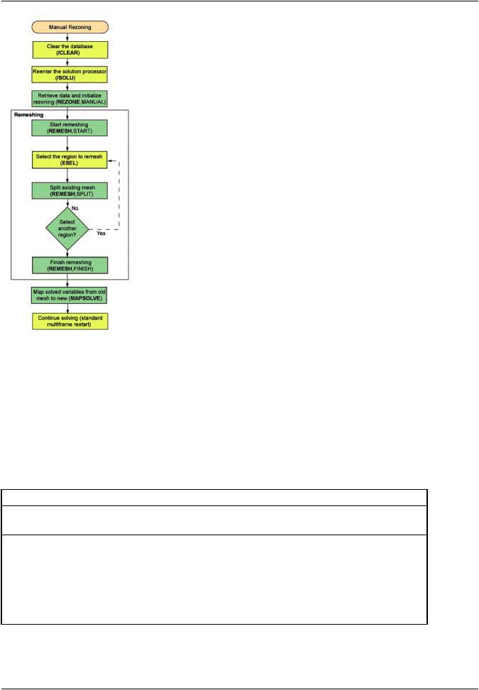
4.3.2. Key Commands Used in Rezoning
Following is a description of key commands used in the rezoning process and provides supplemental information to the rezoning process flowcharts.
Command |
Description |
Rezoning Comments |
|
|
|
/CLEAR |
Clears the data- |
Always clear the database first, before reentering the solu- |
|
base |
tion processor (/SOLU) and starting the rezoning process. |
REZONE |
Initiates rezon- |
When you initiate rezoning, the program verifies that the |
|
ing |
necessary files (.rdb, .rst, .rxxx, and .ldhi) exist for |
|
|
the specified substep and rebuilds the data environment |
|
|
at that substep. |
|
|
All nodes are updated to the deformed geometry in |
|
|
preparation for remeshing. |
|
Release 15.0 - © SAS IP, Inc. All rights reserved. - Contains proprietary and confidential information |
96 |
of ANSYS, Inc. and its subsidiaries and affiliates. |