
- •Table of Contents
- •Chapter 1: Probabilistic Design
- •1.1. Understanding Probabilistic Design
- •1.1.1. Traditional (Deterministic) vs. Probabilistic Design Analysis Methods
- •1.1.2. Reliability and Quality Issues
- •1.2. Probabilistic Design Terminology
- •1.3. Using Probabilistic Design
- •1.3.1. Create the Analysis File
- •1.3.1.1. Example Problem Description
- •1.3.1.2. Build the Model Parametrically
- •1.3.1.3. Obtain the Solution
- •1.3.1.4. Retrieve Results and Assign as Output Parameters
- •1.3.1.5. Prepare the Analysis File
- •1.3.2. Establish Parameters for Probabilistic Design Analysis
- •1.3.3. Enter the PDS and Specify the Analysis File
- •1.3.4. Declare Random Input Variables
- •1.3.5. Visualize Random Input Variables
- •1.3.6. Specify Correlations Between Random Variables
- •1.3.7. Specify Random Output Parameters
- •1.3.8. Select a Probabilistic Design Method
- •1.3.8.1. Probabilistic Method Determination Wizard
- •1.3.9. Execute Probabilistic Analysis Simulation Loops
- •1.3.9.1. Probabilistic Design Looping
- •1.3.9.2. Serial Analysis Runs
- •1.3.9.3. PDS Parallel Analysis Runs
- •1.3.9.3.1. Machine Configurations
- •1.3.9.3.1.1. Choosing Slave Machines
- •1.3.9.3.1.2. Using the Remote Shell Option
- •1.3.9.3.1.3. Using the Connection Port Option
- •1.3.9.3.1.4. Configuring the Master Machine
- •1.3.9.3.1.5. Host setup using port option
- •1.3.9.3.1.6. Host and Product selection for a particular analysis
- •1.3.9.3.2. Files Needed for Parallel Run
- •1.3.9.3.3. Controlling Server Processes
- •1.3.9.3.4. Initiate Parallel Run
- •1.3.10. Fit and Use Response Surfaces
- •1.3.10.1. About Response Surface Sets
- •1.3.10.2. Fitting a Response Surface
- •1.3.10.3. Plotting a Response Surface
- •1.3.10.4. Printing a Response Surface
- •1.3.10.5. Generating Monte Carlo Simulation Samples on the Response Surfaces
- •1.3.11. Review Results Data
- •1.3.11.1. Viewing Statistics
- •1.3.11.2. Viewing Trends
- •1.3.11.3. Creating Reports
- •1.4. Guidelines for Selecting Probabilistic Design Variables
- •1.4.1. Choosing and Defining Random Input Variables
- •1.4.1.1. Random Input Variables for Monte Carlo Simulations
- •1.4.1.2. Random Input Variables for Response Surface Analyses
- •1.4.1.3. Choosing a Distribution for a Random Variable
- •1.4.1.3.1. Measured Data
- •1.4.1.3.2. Mean Values, Standard Deviation, Exceedence Values
- •1.4.1.3.3. No Data
- •1.4.1.4. Distribution Functions
- •1.4.2. Choosing Random Output Parameters
- •1.5. Probabilistic Design Techniques
- •1.5.1. Monte Carlo Simulations
- •1.5.1.1. Direct Sampling
- •1.5.1.2. Latin Hypercube Sampling
- •1.5.1.3. User-Defined Sampling
- •1.5.2. Response Surface Analysis Methods
- •1.5.2.1. Central Composite Design Sampling
- •1.5.2.2. Box-Behnken Matrix Sampling
- •1.5.2.3. User-Defined Sampling
- •1.6. Postprocessing Probabilistic Analysis Results
- •1.6.1. Statistical Postprocessing
- •1.6.1.1. Sample History
- •1.6.1.2. Histogram
- •1.6.1.3. Cumulative Distribution Function
- •1.6.1.4. Print Probabilities
- •1.6.1.5. Print Inverse Probabilities
- •1.6.2. Trend Postprocessing
- •1.6.2.1. Sensitivities
- •1.6.2.2. Scatter Plots
- •1.6.2.3. Correlation Matrix
- •1.6.3. Generating an HTML Report
- •1.7. Multiple Probabilistic Design Executions
- •1.7.1. Saving the Probabilistic Design Database
- •1.7.2. Restarting a Probabilistic Design Analysis
- •1.7.3. Clearing the Probabilistic Design Database
- •1.8. Example Probabilistic Design Analysis
- •1.8.1. Problem Description
- •1.8.2. Problem Specifications
- •1.8.2.1. Problem Sketch
- •1.8.3. Using a Batch File for the Analysis
- •1.8.4. Using the GUI for the PDS Analysis
- •Chapter 2: Variational Technology
- •2.1. Harmonic Sweep Using VT Accelerator
- •2.1.1. Structural Elements Supporting Frequency-Dependent Properties
- •2.1.2. Harmonic Sweep for Structural Analysis with Frequency-Dependent Material Properties
- •2.1.2.1. Beam Example
- •Chapter 3: Adaptive Meshing
- •3.1. Prerequisites for Adaptive Meshing
- •3.2. Employing Adaptive Meshing
- •3.3. Modifying the Adaptive Meshing Process
- •3.3.1. Selective Adaptivity
- •3.3.2. Customizing the ADAPT Macro with User Subroutines
- •3.3.2.1. Creating a Custom Meshing Subroutine (ADAPTMSH.MAC)
- •3.3.2.2. Creating a Custom Subroutine for Boundary Conditions (ADAPTBC.MAC)
- •3.3.2.3. Creating a Custom Solution Subroutine (ADAPTSOL.MAC)
- •3.3.2.4. Some Further Comments on Custom Subroutines
- •3.3.3. Customizing the ADAPT Macro (UADAPT.MAC)
- •3.4. Adaptive Meshing Hints and Comments
- •3.5. Where to Find Examples
- •Chapter 4: Rezoning
- •4.1. Benefits and Limitations of Rezoning
- •4.1.1. Rezoning Limitations
- •4.2. Rezoning Requirements
- •4.3. Understanding the Rezoning Process
- •4.3.1. Overview of the Rezoning Process Flow
- •4.3.2. Key Commands Used in Rezoning
- •4.4. Step 1: Determine the Substep to Initiate Rezoning
- •4.5. Step 2. Initiate Rezoning
- •4.6. Step 3: Select a Region to Remesh
- •4.7. Step 4: Perform the Remeshing Operation
- •4.7.1. Choosing a Remeshing Method
- •4.7.1.1. Remeshing Using a Program-Generated New Mesh (2-D)
- •4.7.1.1.1. Creating an Area to Remesh
- •4.7.1.1.2. Using Nodes From the Old Mesh
- •4.7.1.1.3. Hints for Remeshing Multiple Regions
- •4.7.1.1.4. Generating a New Mesh
- •4.7.1.2. Remeshing Using a Generic New Mesh (2-D and 3-D)
- •4.7.1.2.1. Using the REMESH Command with a Generic New Mesh
- •4.7.1.2.2. Requirements for the Generic New Mesh
- •4.7.1.2.3. Using the REGE and KEEP Remeshing Options
- •4.7.1.3. Remeshing Using Manual Mesh Splitting (2-D and 3-D)
- •4.7.1.3.1. Understanding Mesh Splitting
- •4.7.1.3.2. Geometry Details for Mesh Splitting
- •4.7.1.3.3. Using the REMESH Command for Mesh Splitting
- •4.7.1.3.4. Mesh-Transition Options for 2-D Mesh Splitting
- •4.7.1.3.5. Mesh-Transition Options for 3-D Mesh Splitting
- •4.7.1.3.7. Improving Tetrahedral Element Quality via Mesh Morphing
- •4.7.2. Mesh Control
- •4.7.3. Remeshing Multiple Regions at the Same Substep
- •4.8. Step 5: Verify Applied Contact Boundaries, Surface-Effect Elements, Loads, and Boundary Conditions
- •4.8.1. Contact Boundaries
- •4.8.2. Surface-Effect Elements
- •4.8.3. Pressure and Contiguous Displacements
- •4.8.4. Forces and Isolated Applied Displacements
- •4.8.5. Nodal Temperatures
- •4.8.6. Other Boundary Conditions and Loads
- •4.9. Step 6: Automatically Map Variables and Balance Residuals
- •4.9.1. Mapping Solution Variables
- •4.9.2. Balancing Residual Forces
- •4.9.3. Interpreting Mapped Results
- •4.9.4. Handling Convergence Difficulties
- •4.10. Step 7: Perform a Multiframe Restart
- •4.11. Repeating the Rezoning Process if Necessary
- •4.11.1. File Structures for Repeated Rezonings
- •4.12. Postprocessing Rezoning Results
- •4.12.1. The Database Postprocessor
- •4.12.1.1. Listing the Rezoning Results File Summary
- •4.12.1.2. Animating the Rezoning Results
- •4.12.1.3. Using the Results Viewer for Rezoning
- •4.12.2. The Time-History Postprocessor
- •4.13. Rezoning Restrictions
- •4.14. Rezoning Examples
- •4.14.1. Example: Rezoning Using a Program-Generated New Mesh
- •4.14.1.1. Initial Input for the Analysis
- •4.14.1.2. Rezoning Input for the Analysis
- •4.14.2. Example: Rezoning Using a Generic New Mesh
- •4.14.2.1. Initial Input for the Analysis
- •4.14.2.2. Exporting the Distorted Mesh as a CDB File
- •4.14.2.3. Importing the File into ANSYS ICEM CFD and Generating a New Mesh
- •4.14.2.4. Rezoning Using the New CDB Mesh
- •Chapter 5: Mesh Nonlinear Adaptivity
- •5.1. Mesh Nonlinear Adaptivity Benefits, Limitations and Requirements
- •5.1.1. Rubber Seal Simulation
- •5.1.2. Crack Simulation
- •5.2. Understanding the Mesh Nonlinear Adaptivity Process
- •5.2.1. Checking Nonlinear Adaptivity Criteria
- •5.2.1.1. Defining Element Components
- •5.2.1.2. Defining Nonlinear Adaptivity Criteria
- •5.2.1.3. Defining Criteria-Checking Frequency
- •5.3. Mesh Nonlinear Adaptivity Criteria
- •5.3.1. Energy-Based
- •5.3.2. Position-Based
- •5.3.3. Contact-Based
- •5.3.4. Frequency of Criteria Checking
- •5.4. How a New Mesh Is Generated
- •5.5. Convergence at Substeps with the New Mesh
- •5.6. Controlling Mesh Nonlinear Adaptivity
- •5.7. Postprocessing Mesh Nonlinear Adaptivity Results
- •5.8. Mesh Nonlinear Adaptivity Examples
- •5.8.1. Example: Rubber Seal Simulation
- •5.8.2. Example: Crack Simulation
- •Chapter 6: 2-D to 3-D Analysis
- •6.1. Benefits of 2-D to 3-D Analysis
- •6.2. Requirements for a 2-D to 3-D Analysis
- •6.3. Overview of the 2-D to 3-D Analysis Process
- •6.3.1. Overview of the 2-D to 3-D Analysis Process Flow
- •6.3.2. Key Commands Used in 2-D to 3-D Analysis
- •6.4. Performing a 2-D to 3-D Analysis
- •6.4.1. Step 1: Determine the Substep to Initiate
- •6.4.2. Step 2: Initiate the 2-D to 3-D Analysis
- •6.4.3. Step 3: Extrude the 2-D Mesh to the New 3-D Mesh
- •6.4.4. Step 4: Map Solution Variables from 2-D to 3-D Mesh
- •6.4.5. Step 5: Perform an Initial-State-Based 3-D Analysis
- •6.5. 2-D to 3-D Analysis Restrictions
- •Chapter 7: Cyclic Symmetry Analysis
- •7.1. Understanding Cyclic Symmetry Analysis
- •7.1.1. How the Program Automates a Cyclic Symmetry Analysis
- •7.1.2. Commands Used in a Cyclic Symmetry Analysis
- •7.2. Cyclic Modeling
- •7.2.1. The Basic Sector
- •7.2.2. Edge Component Pairs
- •7.2.2.1. CYCOPT Auto Detection Tolerance Adjustments for Difficult Cases
- •7.2.2.2. Identical vs. Dissimilar Edge Node Patterns
- •7.2.2.3. Unmatched Nodes on Edge-Component Pairs
- •7.2.2.4. Identifying Matching Node Pairs
- •7.2.3. Modeling Limitations
- •7.2.4. Model Verification (Preprocessing)
- •7.3. Solving a Cyclic Symmetry Analysis
- •7.3.1. Understanding the Solution Architecture
- •7.3.1.1. The Duplicate Sector
- •7.3.1.2. Coupling and Constraint Equations (CEs)
- •7.3.1.3. Non-Cyclically Symmetric Loading
- •7.3.1.3.1. Specifying Non-Cyclic Loading
- •7.3.1.3.2. Commands Affected by Non-Cyclic Loading
- •7.3.1.3.3. Plotting and Listing Non-Cyclic Boundary Conditions
- •7.3.1.3.4. Graphically Picking Non-Cyclic Boundary Conditions
- •7.3.2. Solving a Static Cyclic Symmetry Analysis
- •7.3.3. Solving a Modal Cyclic Symmetry Analysis
- •7.3.3.1. Understanding Harmonic Index and Nodal Diameter
- •7.3.3.2. Solving a Stress-Free Modal Analysis
- •7.3.3.3. Solving a Prestressed Modal Analysis
- •7.3.3.4. Solving a Large-Deflection Prestressed Modal Analysis
- •7.3.3.4.1. Solving a Large-Deflection Prestressed Modal Analysis with VT Accelerator
- •7.3.4. Solving a Linear Buckling Cyclic Symmetry Analysis
- •7.3.5. Solving a Harmonic Cyclic Symmetry Analysis
- •7.3.5.1. Solving a Full Harmonic Cyclic Symmetry Analysis
- •7.3.5.1.1. Solving a Prestressed Full Harmonic Cyclic Symmetry Analysis
- •7.3.5.2. Solving a Mode-Superposition Harmonic Cyclic Symmetry Analysis
- •7.3.5.2.1. Perform a Static Cyclic Symmetry Analysis to Obtain the Prestressed State
- •7.3.5.2.2. Perform a Linear Perturbation Modal Cyclic Symmetry Analysis
- •7.3.5.2.3. Restart the Modal Analysis to Create the Desired Load Vector from Element Loads
- •7.3.5.2.4. Obtain the Mode-Superposition Harmonic Cyclic Symmetry Solution
- •7.3.5.2.5. Review the Results
- •7.3.6. Solving a Magnetic Cyclic Symmetry Analysis
- •7.3.7. Database Considerations After Obtaining the Solution
- •7.3.8. Model Verification (Solution)
- •7.4. Postprocessing a Cyclic Symmetry Analysis
- •7.4.1. General Considerations
- •7.4.1.1. Using the /CYCEXPAND Command
- •7.4.1.1.1. /CYCEXPAND Limitations
- •7.4.1.2. Result Coordinate System
- •7.4.2. Modal Solution
- •7.4.2.1. Real and Imaginary Solution Components
- •7.4.2.2. Expanding the Cyclic Symmetry Solution
- •7.4.2.3. Applying a Traveling Wave Animation to the Cyclic Model
- •7.4.2.4. Phase Sweep of Repeated Eigenvector Shapes
- •7.4.3. Static, Buckling, and Full Harmonic Solutions
- •7.4.4. Mode-Superposition Harmonic Solution
- •7.5. Example Modal Cyclic Symmetry Analysis
- •7.5.1. Problem Description
- •7.5.2. Problem Specifications
- •7.5.3. Input File for the Analysis
- •7.5.4. Analysis Steps
- •7.6. Example Buckling Cyclic Symmetry Analysis
- •7.6.1. Problem Description
- •7.6.2. Problem Specifications
- •7.6.3. Input File for the Analysis
- •7.6.4. Analysis Steps
- •7.6.5. Solve For Critical Strut Temperature at Load Factor = 1.0
- •7.7. Example Harmonic Cyclic Symmetry Analysis
- •7.7.1. Problem Description
- •7.7.2. Problem Specifications
- •7.7.3. Input File for the Analysis
- •7.7.4. Analysis Steps
- •7.8. Example Magnetic Cyclic Symmetry Analysis
- •7.8.1. Problem Description
- •7.8.2. Problem Specifications
- •7.8.3. Input file for the Analysis
- •Chapter 8: Rotating Structure Analysis
- •8.1. Understanding Rotating Structure Dynamics
- •8.2. Using a Stationary Reference Frame
- •8.2.1. Campbell Diagram
- •8.2.2. Harmonic Analysis for Unbalance or General Rotating Asynchronous Forces
- •8.2.3. Orbits
- •8.3. Using a Rotating Reference Frame
- •8.4. Choosing the Appropriate Reference Frame Option
- •8.5. Example Campbell Diagram Analysis
- •8.5.1. Problem Description
- •8.5.2. Problem Specifications
- •8.5.3. Input for the Analysis
- •8.5.4. Analysis Steps
- •8.6. Example Coriolis Analysis
- •8.6.1. Problem Description
- •8.6.2. Problem Specifications
- •8.6.3. Input for the Analysis
- •8.6.4. Analysis Steps
- •8.7. Example Unbalance Harmonic Analysis
- •8.7.1. Problem Description
- •8.7.2. Problem Specifications
- •8.7.3. Input for the Analysis
- •8.7.4. Analysis Steps
- •Chapter 9: Submodeling
- •9.1. Understanding Submodeling
- •9.1.1. Nonlinear Submodeling
- •9.2. Using Submodeling
- •9.2.1. Create and Analyze the Coarse Model
- •9.2.2. Create the Submodel
- •9.2.3. Perform Cut-Boundary Interpolation
- •9.2.4. Analyze the Submodel
- •9.3. Example Submodeling Analysis Input
- •9.3.1. Submodeling Analysis Input: No Load-History Dependency
- •9.3.2. Submodeling Analysis Input: Load-History Dependency
- •9.4. Shell-to-Solid Submodels
- •9.5. Where to Find Examples
- •Chapter 10: Substructuring
- •10.1. Benefits of Substructuring
- •10.2. Using Substructuring
- •10.2.1. Step 1: Generation Pass (Creating the Superelement)
- •10.2.1.1. Building the Model
- •10.2.1.2. Applying Loads and Creating the Superelement Matrices
- •10.2.1.2.1. Applicable Loads in a Substructure Analysis
- •10.2.2. Step 2: Use Pass (Using the Superelement)
- •10.2.2.1. Clear the Database and Specify a New Jobname
- •10.2.2.2. Build the Model
- •10.2.2.3. Apply Loads and Obtain the Solution
- •10.2.3. Step 3: Expansion Pass (Expanding Results Within the Superelement)
- •10.3. Sample Analysis Input
- •10.4. Top-Down Substructuring
- •10.5. Automatically Generating Superelements
- •10.6. Nested Superelements
- •10.7. Prestressed Substructures
- •10.7.1. Static Analysis Prestress
- •10.7.2. Substructuring Analysis Prestress
- •10.8. Where to Find Examples
- •Chapter 11: Component Mode Synthesis
- •11.1. Understanding Component Mode Synthesis
- •11.1.1. CMS Methods Supported
- •11.1.2. Solvers Used in Component Mode Synthesis
- •11.2. Using Component Mode Synthesis
- •11.2.1. The CMS Generation Pass: Creating the Superelement
- •11.2.2. The CMS Use and Expansion Passes
- •11.2.3. Superelement Expansion in Transformed Locations
- •11.2.4. Plotting or Printing Mode Shapes
- •11.3. Example Component Mode Synthesis Analysis
- •11.3.1. Problem Description
- •11.3.2. Problem Specifications
- •11.3.3. Input for the Analysis: Fixed-Interface Method
- •11.3.4. Analysis Steps: Fixed-Interface Method
- •11.3.5. Input for the Analysis: Free-Interface Method
- •11.3.6. Analysis Steps: Free-Interface Method
- •11.3.7. Input for the Analysis: Residual-Flexible Free-Interface Method
- •11.3.8. Analysis Steps: Residual-Flexible Free-Interface Method
- •11.3.9. Example: Superelement Expansion in a Transformed Location
- •11.3.9.1. Analysis Steps: Superelement Expansion in a Transformed Location
- •11.3.10. Example: Reduce the Damping Matrix and Compare Full and CMS Results with RSTMAC
- •Chapter 12: Rigid-Body Dynamics and the ANSYS-ADAMS Interface
- •12.1. Understanding the ANSYS-ADAMS Interface
- •12.2. Building the Model
- •12.3. Modeling Interface Points
- •12.4. Exporting to ADAMS
- •12.4.1. Exporting to ADAMS via Batch Mode
- •12.4.2. Verifying the Results
- •12.5. Running the ADAMS Simulation
- •12.6. Transferring Loads from ADAMS
- •12.6.1. Transferring Loads on a Rigid Body
- •12.6.1.1. Exporting Loads in ADAMS
- •12.6.1.2. Importing Loads
- •12.6.1.3. Importing Loads via Commands
- •12.6.1.4. Reviewing the Results
- •12.6.2. Transferring the Loads of a Flexible Body
- •12.7. Methodology Behind the ANSYS-ADAMS Interface
- •12.7.1. The Modal Neutral File
- •12.7.2. Adding Weak Springs
- •12.8. Example Rigid-Body Dynamic Analysis
- •12.8.1. Problem Description
- •12.8.2. Problem Specifications
- •12.8.3. Command Input
- •Chapter 13: Element Birth and Death
- •13.1. Elements Supporting Birth and Death
- •13.2. Understanding Element Birth and Death
- •13.3. Element Birth and Death Usage Hints
- •13.3.1. Changing Material Properties
- •13.4. Using Birth and Death
- •13.4.1. Build the Model
- •13.4.2. Apply Loads and Obtain the Solution
- •13.4.2.1. Define the First Load Step
- •13.4.2.1.1. Sample Input for First Load Step
- •13.4.2.2. Define Subsequent Load Steps
- •13.4.2.2.1. Sample Input for Subsequent Load Steps
- •13.4.3. Review the Results
- •13.4.4. Use Analysis Results to Control Birth and Death
- •13.4.4.1. Sample Input for Deactivating Elements
- •13.5. Where to Find Examples
- •Chapter 14: User-Programmable Features and Nonstandard Uses
- •14.1. User-Programmable Features (UPFs)
- •14.1.1. Understanding UPFs
- •14.1.2. Types of UPFs Available
- •14.2. Nonstandard Uses of the ANSYS Program
- •14.2.1. What Are Nonstandard Uses?
- •14.2.2. Hints for Nonstandard Use of ANSYS
- •Chapter 15: State-Space Matrices Export
- •15.1. State-Space Matrices Based on Modal Analysis
- •15.1.1. Examples of SPMWRITE Command Usage
- •15.1.2. Example of Reduced Model Generation in ANSYS and Usage in Simplorer
- •15.1.2.1. Problem Description
- •15.1.2.2. Problem Specifications
- •15.1.2.3. Input File for the Analysis
- •Chapter 16: Soil-Pile-Structure Analysis
- •16.1. Soil-Pile-Structure Interaction Analysis
- •16.1.1. Automatic Pile Subdivision
- •16.1.2. Convergence Criteria
- •16.1.3. Soil Representation
- •16.1.4. Mudslides
- •16.1.5. Soil-Pile Interaction Results
- •16.1.5.1. Displacements and Reactions
- •16.1.5.2. Forces and Stresses
- •16.1.5.3. UNITY Check Data
- •16.2. Soil Data Definition and Examples
- •16.2.1. Soil Profile Data Definition
- •16.2.1.1. Mudline Position Definition
- •16.2.1.2. Common Factors for P-Y, T-Z Curves
- •16.2.1.3. Horizontal Soil Properties (P-Y)
- •16.2.1.3.1. P-Y curves defined explicitly
- •16.2.1.3.2. P-Y curves generated from given soil properties
- •16.2.1.4. Vertical Soil Properties (T-Z)
- •16.2.1.4.1. T-Z curves defined explicitly
- •16.2.1.4.2. T-Z curves generated from given soil properties
- •16.2.1.5. End Bearing Properties (ENDB)
- •16.2.1.5.1. ENDB curve defined explicitly
- •16.2.1.5.2. ENDB curves generated from given soil properties
- •16.2.1.6. Mudslide Definition
- •16.2.2. Soil Data File Examples
- •16.2.2.1. Example 1: Constant Linear Soil
- •16.2.2.2. Example 2: Non-Linear Soil
- •16.2.2.3. Example 3: Soil Properties Defined in 5 Layers
- •16.2.2.4. Example 4: Soil Properties Defined in 5 Layers with Mudslide
- •16.3. Performing a Soil-Pile Interaction Analysis
- •16.3.2. Mechanical APDL Component System Example
- •16.3.3. Static Structural Component System Example
- •16.4. Soil-Pile-Structure Results
- •16.5. References
- •Chapter 17: Coupling to External Aeroelastic Analysis of Wind Turbines
- •17.1. Sequential Coupled Wind Turbine Solution in Mechanical APDL
- •17.1.1. Procedure for a Sequentially Coupled Wind Turbine Analysis
- •17.1.2. Output from the OUTAERO Command
- •Chapter 18: Applying Ocean Loading from a Hydrodynamic Analysis
- •18.1. How Hydrodynamic Analysis Data Is Used
- •18.2. Hydrodynamic Load Transfer with Forward Speed
- •18.3. Hydrodynamic Data File Format
- •18.3.1. Comment (Optional)
- •18.3.2. General Model Data
- •18.3.3. Hydrodynamic Surface Geometry
- •18.3.4. Wave Periods
- •18.3.5. Wave Directions
- •18.3.6. Panel Pressures
- •18.3.7. Morison Element Hydrodynamic Definition
- •18.3.8. Morison Element Wave Kinematics Definition
- •18.3.9. RAO Definition
- •18.3.10. Mass Properties
- •18.4. Example Analysis Using Results from a Hydrodynamic Diffraction Analysis
- •Index
- •ОГЛАВЛЕНИЕ
- •ВВЕДЕНИЕ
- •1.1. Методология проектирования технологических объектов
- •1.2. Компьютерные технологии проектирования
- •1.3. Системы автоматизированного проектирования в технике
- •1.4. Системы инженерного анализа
- •2.2.1. Создание и сохранение чертежа
- •2.2.2. Изменение параметров чертежа
- •2.2.3. Заполнение основной надписи
- •2.2.4. Создание нового вида. Локальная система координат
- •2.2.5. Вычерчивание изображения прокладки
- •2.2.6. Простановка размеров
- •2.2.7. Ввод технических требований
- •2.2.8. Задание материала изделия
- •2.3. Сложные разрезы в чертеже детали «Основание»
- •2.3.1. Подготовка чертежа
- •Cохранить документ.
- •2.3.2. Черчение по сетке из вспомогательных линий
- •2.3.3. Изображение разрезов
- •2.4. Чертежи общего вида при проектировании
- •3.1. Интерфейс программы
- •3.2. Общее представление о трехмерном моделировании
- •3.3. Основные операции геометрического моделирования
- •3.3.1. Операция выдавливания
- •3.3.2. Операция вращения
- •3.3.3. Кинематическая операция
- •3.3.4. Построение тела по сечениям
- •3.4. Операции конструирования
- •3.4.1. Построение фасок и скруглений
- •3.4.2. Построение уклона
- •3.4.3. Сечение модели плоскостью
- •3.4.4. Сечение по эскизу
- •3.4.5. Создание моделей-сборок
- •3.5. Разработка электронных 3D-моделей тепловых устройств
- •3.5.1. Электронные модели в ЕСКД
- •3.5.2. Электронные «чертежи» в ЕСКД
- •3.5.4. Электронная модель сборочного изделия «Газовая горелка»
- •ГЛАВА 4. ИНЖЕНЕРНЫЙ АНАЛИЗ ГАЗОДИНАМИКИ И ТЕПЛООБМЕНА В ANSYS CFX
- •4.1. Область применения ANSYS CFX
- •4.2. Особенности вычислительного процесса в ANSYS CFX
- •4.3. Программы, используемые при расчетах в ANSYS CFX
- •4.4. Организация процесса вычислений в среде пакета Workbench
- •4.4.1. Графический интерфейс пользователя
- •5.1. Постановка теплофизических задач в ANSYS Multiphysics
- •5.2. Решение задач в пакете ANSYS Multiphysics
- •5.2.1. Графический интерфейс пользователя
- •5.2.2. Этапы препроцессорной подготовки решения
- •5.2.3. Этап получения решения и постпроцессорной обработки результатов
- •5.3.5. Нестационарный теплообмен. Нагрев пластины в печи с жидким теплоносителем
- •5.4.1. Температурные напряжения при нагреве
- •БИБЛИОГРАФИЧЕСКИЙ СПИСОК

vk.com/club152685050 | vk.com/id446425943 |
Probabilistic Design Techniques |
1 |
1 |
1 |
1.619379209e+000 |
2.364528435e-001 |
1.470789050e+000 |
1 |
1 |
2 |
2.237676559e-001 5.788049712e-001 1.821263115e+000 |
||
1 |
1 |
3 |
7.931615474e+000 |
8.278689033e-001 |
2.170793522e+000 |
.. .. |
.. |
... |
... |
... |
|
.. .. |
.. |
... |
... |
... |
|
1 |
1 |
98 |
1.797221666e+000 |
3.029471373e-001 |
1.877701081e+000 |
1 |
1 |
99 |
1.290815540e+001 |
9.271606216e-001 |
2.091047328e+000 |
1 |
1 |
100 |
4.699281922e+000 |
6.526505821e-001 |
1.901013985e+000 |
1.5.2. Response Surface Analysis Methods
For response surface analysis, you can choose from three sampling methods: Central Composite Design, Box-Behnken Matrix, and user-defined.
Response surface methods are based on the fundamental assumption that the influence of the random input variables on the random output parameters can be approximated by mathematical function. Hence, Response Surface Methods locate the sample points in the space of random input variables such that an appropriate approximation function can be found most efficiently; typically, this is a quadratic
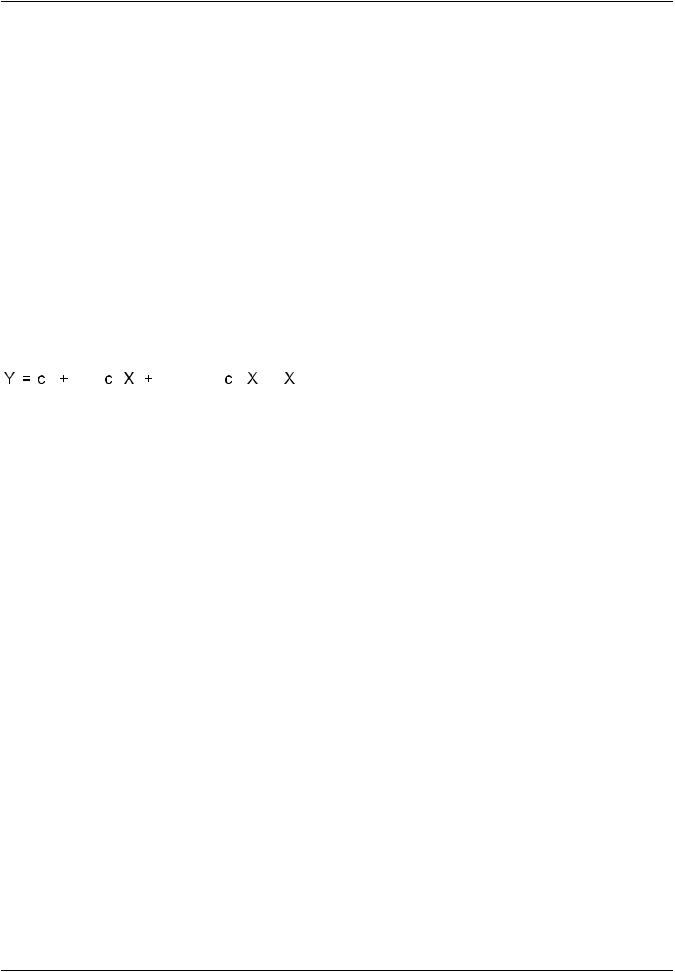
polynomial. In this case the approximation function ^ is described by |
|||||
|
|
|
|
|
Y |
|
NRV |
NRV NRV |
|
|
|
|
∑ |
∑ |
∑ |
|
|
0 |
i i |
|
ij |
i |
j |
|
i =1 |
i =1 |
j = i |
|
|
where c0 is the coefficient of the constant term, ci, i = 1,...NRV are the coefficients of the linear terms and cij, i = 1,...NRV and j = i, ...,NRV are the coefficients of the quadratic terms. To evaluate these coefficients a regression analysis is used and the coefficients are usually evaluated such that the sum of squared differences between the true simulation results and the values of the approximation function is minimized.
Hence, a response surface analysis consists of two steps:
1.Performing the simulation loops to calculate the values of the random output parameters that correspond to the sample points in the space of random input variables.
2.Performing a regression analysis to derive the terms and the coefficients of the approximation function.
The fundamental idea of Response Surface Methods is that once the coefficients of a suitable approximation function are found, then we can directly use the approximation function instead of looping through the finite element model. To perform a finite element analysis might require minutes to hours of computation time; in contrast, evaluating a quadratic function requires only a fraction of a second. Hence, if using the approximation function, we can afford to evaluate the approximated response parameter thousands of times.
A quadratic polynomial is sufficient in many cases of engineering analysis (for example, the evaluation of the thermal stress mentioned above). For that evaluation, the Young's modulus and the thermal expansion coefficient both have a linear effect on the thermal stresses, which is taken into account in a quadratic approximation by the mixed quadratic terms. However, there are cases where a quadratic approximation is not sufficient; for example, if the finite element results are used to calculate the lifetime of a component. For this evaluation, the lifetime typically shows an exponential behavior with respect
to the input parameters; thus the lifetime results cannot be directly or sufficiently described by a quadratic polynomial. But often, if you apply a logarithmic transformation to the lifetime results, then these transformed values can be approximated by a quadratic polynomial. The ANSYS PDS offers a
Release 15.0 - © SAS IP, Inc. All rights reserved. - Contains proprietary and confidential information |
|
of ANSYS, Inc. and its subsidiaries and affiliates. |
55 |

vk.com/club152685050Probabi istic Design | vk.com/id446425943
variety of transformation functions that you can apply to the response parameters, and the logarithmic transformation function is one of them.
Assuming the approximation function is suitable for your problem, the advantages of the Response Surface Method are:
•It often requires fewer simulation loops than the Monte Carlo Simulation method.
•It can evaluate very low probability levels. This is something the Monte Carlo Simulation method cannot do unless you perform a great number of simulation loops.
•The goodness-of-fit parameters tell you how good the approximation function is (in other words, how accurate the approximation function is that describes your "true" response parameter values). The goodness-of-fit parameters can warn you if the approximation function is insufficient.
•The individual simulation loops are inherently independent (the individual simulation loops do not depend on the results of any other simulation loops). This makes Response Surface Method an ideal candidate for parallel processing.
The disadvantages of the Response Surface Method are:
•The number of required simulation loops depends on the number of random input variables. If you have a very large number of random input variables (hundreds or even thousands), then a probabilistic analysis using Response Surface Methods would be impractical.
•This method is not usually suitable for cases where a random output parameter is a non-smooth function of the random input variables. For example, a non-smooth behavior is given if you observe a sudden jump of the output parameter value even if the values for the random input variables vary only slightly. This typically occurs if you have instability in your model (such as bulking). The same might happen if the model includes a sharp nonlinearity such as a linear-elastic-ideal-plastic material behavior. Or, if you are analyzing a contact problem, where only a slight variation in your random input variables can change the contact situation from contact to non-contact or vice versa, then you also might have problems using the Response Surface Method.
Note
To use Response Surface Methods, the random output parameters must be smooth and continuous functions of the involved random input variables. Do not use Response Surface Methods if this condition is not satisfied.
1.5.2.1. Central Composite Design Sampling
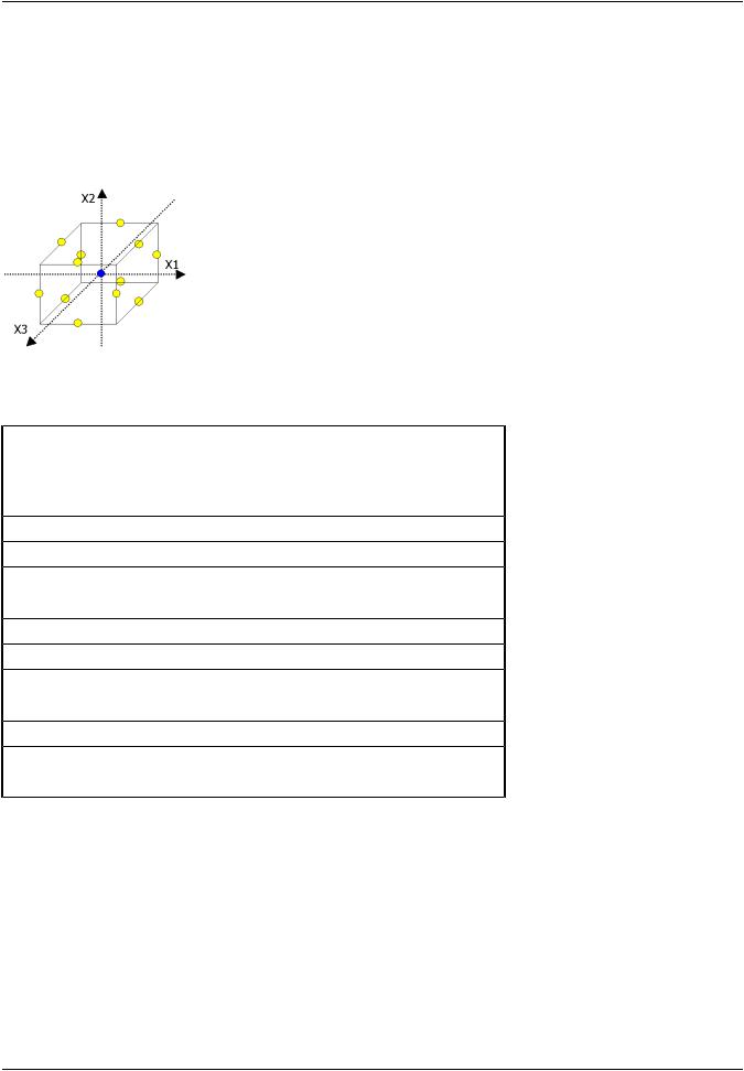
A central composite design consists of a central point, the N axis point plus 2N-f factorial points located at the corners of an N-dimensional hypercube. Here, N is the number of random input variables and f is the fraction of the factorial part of the central composite design. A fraction f = 0 is a called a full factorial design, f = 1 gives a half-factorial design, and so on. The PDS gradually increases the fraction
f as you increase the number of random input variables. This keeps the number of simulation loops reasonable. The fraction f is automatically evaluated such that a resolution V design is always maintained. A resolution V design is a design where none of the second order terms of the approximation function are confined with each other. This ensures a reasonable accuracy for the evaluation of the coefficients
of the second order terms.
The locations of the sampling points for a problem with three random input variables is illustrated below.
|
Release 15.0 - © SAS IP, Inc. All rights reserved. - Contains proprietary and confidential information |
56 |
of ANSYS, Inc. and its subsidiaries and affiliates. |

vk.com/club152685050 | vk.com/id446425943 |
Probabilistic Design Techniques |
Figure 1.9: Locations of Sampling Points for Problem with Three Input Variables for CCD
The number of sample points (simulation loops) required for a central composite design as a function of the number of random input variables is given in the table below:
Number of ranNumber of coefficients in |
Factorial num- |
Number sample |
|
dom input vari- a quadratic function (with |
ber f |
points (simulation |
|
ables |
cross-terms) |
|
loops) |
1 |
3 |
N/A |
N/A |
2 |
6 |
0 |
9 |
3 |
10 |
0 |
15 |
4 |
15 |
0 |
25 |
5 |
21 |
1 |
27 |
6 |
28 |
1 |
45 |
7 |
36 |
1 |
79 |
8 |
45 |
2 |
81 |
9 |
55 |
2 |
147 |
10 |
66 |
3 |
149 |
11 |
78 |
4 |
151 |
12 |
91 |
4 |
281 |
13 |
105 |
5 |
283 |
14 |
120 |
6 |
285 |
15 |
136 |
7 |
287 |
16 |
153 |
8 |
289 |
17 |
171 |
9 |
291 |
18 |
190 |
9 |
549 |
19 |
210 |
10 |
551 |
20 |
231 |
11 |
553 |
To use the Response Surface Method with a Central Composite Design, do the following:
Command(s): PDMETH,RSM,CCD PDDOEL,Name,CCD,...
GUI: Main Menu> Prob Design> Prob Method> Response Surface
PDDOEL allows you to specify design of experiment options.
See the Mechanical APDL Theory Reference for more details.
Release 15.0 - © SAS IP, Inc. All rights reserved. - Contains proprietary and confidential information |
|
of ANSYS, Inc. and its subsidiaries and affiliates. |
57 |

vk.com/club152685050Probabi istic Design | vk.com/id446425943
1.5.2.2. Box-Behnken Matrix Sampling
A Box-Behnken Design consists of a central point plus the midpoints of each edge of an N-dimensional hypercube.
The location of the sampling points for a problem with three random input variables is illustrated below.
Figure 1.10: Location of Sampling Points for Problem with Three Input Variables for BBM
The number of sample points (simulation loops) required for a Box-Behnken design as a function of the number of random input variables is given in the table below:
Number of ranNumber of coefficients in |
Number sample |
|
dom input vari- a quadratic function (with |
points (simulation |
|
ables |
cross-terms) |
loops) |
1 |
|
N/A |
2 |
6 |
N/A |
3 |
10 |
12 |
4 |
15 |
25 |
5 |
21 |
41 |
6 |
28 |
49 |
7 |
36 |
57 |
8 |
45 |
65 |
9 |
55 |
121 |
10 |
66 |
161 |
11 |
78 |
177 |
12 |
91 |
193 |
To use Response Surface Analysis with the Box-Behnken design option, do the following:
Command(s): PDMETH,RSM,BBM PDDOEL,Name,BBM,...
GUI: Main Menu> Prob Design> Prob Method> Response Surface
PDDOEL allows you to specify design of experiment options.
See the Mechanical APDL Theory Reference for more details.
1.5.2.3. User-Defined Sampling
For this method, you provide the file containing the samples.
|
Release 15.0 - © SAS IP, Inc. All rights reserved. - Contains proprietary and confidential information |
58 |
of ANSYS, Inc. and its subsidiaries and affiliates. |